2025-07-14 21:35:35
Newton’s method is a simple and efficient method for finding the roots of equations, provided you start close enough to the root. But determining the set of starting points that converge to a given root, or converge at all, can be very complicated.
In one case it is easy to completely classify where points converge. Suppose you have a quadratic polynomial p(x) with distinct roots a and b in the complex plane. The line perpendicular to the line between a and b is a sort of continental divide, splitting the plane into two watersheds. If you start Newton’s method at any point on a root’s side of the line, it will converge to that root.
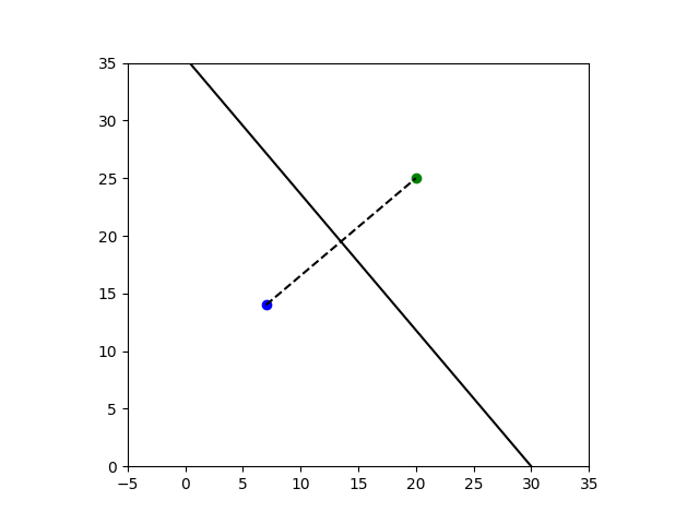
To illustrate this, we will set a = 7 + 14i and b = 20 + 25i, and use Newton’s method to find the roots of
p(z) = (z − a)(z − b).
You can start far from the root and still converge, which isn’t typical but is the case for quadratic polynomials.
And the point you’ll converge to is determined by which side of the continental divide you start on. For example, the following code shows that if you start at 1000 + 2000i you will converge to 20 + 25i.
a = 7 + 14j
b = 20 + 25j

p      = lambda z: (z - a)*(z - b)
pprime = lambda z: (z - a) + (z - b)
newton = lambda z: z - p(z)/pprime(z)

z = 1000 + 2000j
for _ in range(12):
    z = newton(z)
    print(z)
If you’re not familiar with Python, note that it uses j for the imaginary unit. Here’s why.
Things are more complicated if you start Newton’s method exactly on the line dividing the two watersheds. The method will not converge. There is a dense set of starting points on the line that will cycle through a finite number of points. And there is a dense set of points that lead to division by zero. (See HAKMEM, item 3.)
2025-07-13 20:41:47
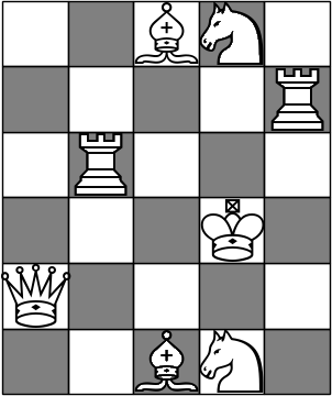
Here’s another little chess puzzle by Martin Gardner, taken from this paper.
The task is to place all the pieces—king, queen, two bishops, two knights, and two rooks—on a 6 × 5 chessboard, with the requirement that the two bishops be on opposite colored squares and no piece is attacking another.
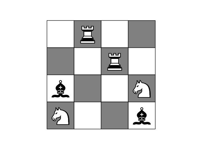
Here is a solution.
The post All pieces on a small chessboard first appeared on John D. Cook.2025-07-10 00:44:26
Our team started working within Nvidia in early 2009 at the beginning of the ORNL Titan project. Our Nvidia contacts dealt with applications, libraries, programming environment and performance optimization. First impressions were that their technical stance on issues was very reasonable. One obscure example: in a C++ CUDA kernel were you allowed to use “enums,” and the answer would be, of course, yes, we would allow that. This was unlike some other companies that might have odd and cumbersome programming restrictions in their parallel programming models (though by now this has become a harder problem for Nvidia since there are so many software products a user might want to interoperate).
Another example, with a colleague at Nvidia on the C++ standards committee, to whom I mentioned, it might be too early to lock this certain feature design into the standard since hardware designs are still rapidly changing. His response was, Oh, yes, we think exactly the same thing. So in short, their software judgments and decisions generally seem to be well thought out, reasonable and well informed. It sounds simple, but it is amazing how many companies have gotten this wrong.
Nvidia has made good strategic decisions. In the 2013 time frame, Intel was becoming a competitive threat with the Xeon Phi processor. Intel was several times larger than Nvidia with huge market dominance. In response, Nvidia formed a partnership with IBM–itself several times larger than Intel at the time. This came to fruition in the ORNL Summit system in 2018. In the meantime, the Xeon Phi’s OpenMP programming model, though standards-based, turned out to be difficult to write optimized code for, and Nvidia CUDA captured market share dominance of accelerated user software. Intel eventually dropped the Xeon Phi product line.
In the early 2000s, Nvidia went all-in on CUDA. I’ve heard some project teams say they would never use CUDA, because it is nonstandard and too low-level. Many have turned back on this decision. Of course, it is often possible to write an abstraction layer on top of CUDA to make it easier to use and maintain. Also newer programming models like Kokkos can be helpful.
Nvidia also made a prescient decision early to bet big on AI. A little later they decided to go all in on developing a huge number of software libraries is to enable access to many new markets. A huge moat. AMD is trying hard to improve their software processes and catch up.
On the downside, Nvidia high prices are upsetting to many, from gamers to buyers of the world’s largest HPC systems. Competition from AMD and others is a good thing.
And Nvidia marketing speak is sometimes confusing. A comparison was once made claiming that a four GPU system was more powerful than one of the world’s top CPU-only supercomputers on a very specific science problem. I’d like to see the details of that comparison. Also, different figures are being given on how long it took to stand up xAI’s Colossus supercomputer, from 19 days to 122 days. One has to dig a little to find out what these figures mean. Also it was widely reported last year that the GB200 NVL72 GPU was “30 times faster” than H100, but this only refers to certain operations, not key performance measures like flops per watt.
Those are my takes. For more perspectives, see Tae Kim’s excellent book, The Nvidia Way, or this interview.
Thoughts on Nvidia? Please leave in the comments.
The post Experiences with Nvidia first appeared on John D. Cook.
2025-07-08 08:59:41
The previous post mentioned Legendre polynomials. This post will give a brief introduction to these polynomials and a couple hints of how they are used in applications.
One way to define the Legendre polynomials is as follows.
The middle bullet point means
![]()
if m ≠ n. The requirement that each Pk is orthogonal to each of its predecessors determines Pk up to a constant, and the condition Pk(1) = 1 determines this constant.
Here’s a plot of the first few Legendre polynomials.
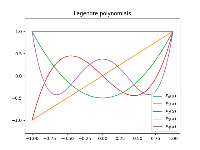
There’s an interesting pattern that appears in the white space of a graph like the one above when you plot a large number of Legendre polynomials. See this post.
The Legendre polynomial Pk(x) satisfies Legendre’s differential equation; that’s what motivated them.
![]()
This differential equation comes up in the context of spherical harmonics.
Next I’ll describe a geometric motivation for the Legendre polynomials. Suppose you have a triangle with one side of unit length and two longer sides of length r and y.
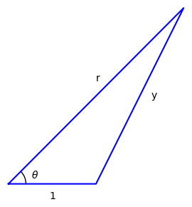
You can find y in terms of r by using the law of cosines:
![]()
But suppose you want to find 1/y in terms of a series in 1/r. (This may seem like an arbitrary problem, but it comes up in applications.) Then the Legendre polynomials give you the coefficients of the series.
![]()
Source: Keith Oldham et al. An Atlas of Functions. 2nd edition.
2025-07-07 19:36:05
To first approximation, a satellite orbiting the earth moves in an elliptical orbit. That’s what would get from solving the two-body problem: two point masses orbiting their common center of mass, subject to no forces other than their gravitational attraction to each other.
But the earth is not a point mass. Neither is a satellite, though that’s much less important. The fact that the earth is not exactly a sphere but rather an oblate spheroid is the root cause of the J2 effect.
The J2 effect is the largest perturbation of a satellite orbit from a simple elliptical orbit, at least for satellites in low earth orbit (LEO) and medium earth orbit (MEO). The J2 effect is significant for satellites in higher orbits, though third body effects are larger.
Legendre showed that the gravitational potential of an axially symmetric planet is given by

Here (r, φ) are spherical coordinates. There’s no θ term because we assume the planet, and hence its gravitational potential, is axially symmetric, i.e. independent of θ. The term req is the equatorial radius of the planet. The Pk are Legendre polynomials.
For a moderately oblate planet, like the one we live on, the J2 coefficient is much larger than the others, and neglecting the rest of the coefficients gives a good approximation [1].
Here are the first few coefficients for Earth [2].

Note that J2 is three orders of magnitude smaller than 1, and so the J2 effect is small. And yet it matters a great deal. The longitude of the point at which a satellite crosses the equatorial plane may vary a few degrees per day. The rate of precession is approximately proportional to J2.
The value of J2 for Mars is about twice that of Earth (0.001960454). The largest J2 in our solar system is Neptune, which is about three times that of Earth (0.003411).
There are many factors left out of the assumptions of the two body problem. The J2 effect doesn’t account for everything that has been left out, but it’s the first refinement.
[1] Legendre discovered/invented what we now call the Legendre polynomials in the course of calculating the gravitational potential above. I assume the convention of using J for the coefficients goes back to Legendre.
[2] Richard H. Battin. An Introduction to the Mathematics and Methods of Astrodynamics, Revised Edition, 1999.
The post The biggest perturbation of satellite orbits first appeared on John D. Cook.2025-07-06 02:33:08
Suppose you have a radio transmitter T and a receiver R with a clear line of sight between them. Some portion the signal received at R will come straight from T. But some portion will have bounced off some obstacle, such as the ground.
The reflected radio waves will take a longer path than the waves that traveled straight from T to R. The worst case for reception is when the waves traveling a longer path arrive half a period later, i.e. 180° out of phase, canceling out part of the signal that was received directly.
We’d like to describe the region of space that needs to be empty in order to eliminate destructive interference, i.e. signals 180° out of phase. Suppose T and R are a distance d apart and the wavelength of your signal is λ. An obstacle at a location P can cause signals to arrive exactly out of phase if the distance from T to P plus the distance from P to R is d + λ/2.
So we’re looking for the set of all points such that the sum of their distances to fixes points is a constant. This is the nails-and-string description of an ellipse, where the nails are a distance d apart and the string has length d + λ/2.
That would be a description of the region if we were limited to a plane, such as a plane perpendicular to the ground and containing the transmitter and receiver. But signals could reflect off an obstacle that’s outside this plane. So now we need to imagine being able to move the string in three dimensions. We still get all the points we’d get if we were restricted to a plane, but we also get their rotation about the axis running between T and R.
The region we’re describing is an ellipsoid, known as a Fresnel ellipsoid or Fresnel zone.
Suppose we choose our coordinates so that our transmitter T is located at (0, 0, h) and our receiver R is located at (d, 0, h). We imagine a string of length d + λ/2 with endpoints attached to T and R. We stretch the string so it consists of two straight segments. The set of all possible corners in the string traces out the Fresnel ellipsoid.
If reflected waves are delayed by exactly one period, they reinforce the portion of the signal that arrived directly. Signals delayed by an even multiple of a half-period cause constructive interference, but signals delayed by odd multiples of a half-period cause destructive interference. The odd multiples matter most because we’re more often looking to avoid destructive interference rather than seeking out opportunities for constructive interference.
If you repeat the exercise above with a string of length length d + λ you have another Fresnel ellipsoid. The foci remain the same, i.e. T and R, but this new ellipsoid is bigger since the string is longer. This ellipsoid represents locations where a signal reflected at that point will arrive one period later than a signal traveling straight. Obstacles on the surface of this ellipsoid cause constructive interference.
We can repeat this exercise for a string of length d + nλ/2, where odd values of n correspond to regions of destructive interference. This gives us a set of confocal ellipsoids known as the Fresnel ellipsoids.