2026-06-15 04:35:57

与人闲谈时,但凡提及抖音、快手之类的短视频应用,我总会说,自己从不涉猎,亦不曾注册。
平心而论,我始终觉得,短视频不过是献给忙碌现代人的一剂麻醉。那些被日常琐事填满、仅在罅隙中喘息的灵魂,借片刻光影抚慰疲惫,或是填补突如其来的空虚。可前几日,当我在街头看见连稚子都低头沉浸于抖音之中,忽而惊觉——或许再过几年,那种传统的、从容的闲暇方式,便要彻底消逝了。那一刻我才真正意识到,我们谈论的「闲暇」,早已不是同一种东西。
「闲暇本是稀缺之物。」多少人从晨光微露奔波至夜幕低垂,竟无片刻空闲。闲暇并非时间上的空余,而是一种心境,一种多数人早已遗失的心境。又或者,大多数人的所谓闲暇,不过是日历上那几个被红笔圈出的节假日罢了。他们身在假期,心却仍被未读的消息和待办的事项攥紧,何尝真正歇息过?
短视频恰是这种「伪闲暇」的极致形态。它是一种「放松的异化」——表面上,刷短视频是在放松,实则令大脑时刻处于兴奋状态,无从松弛。它不断尝试用几十秒的光影攫取你的注意力,嘈杂的背景音乐与刻意调高的音量,更是持续施加着心理暗示。算法统治了一切,它比你自己更懂得你的喜好,在滑动屏幕的过程中,将你困于无形的信息孤岛。
正因如此,我始终偏爱另一种活法。
若有片刻空闲,我总喜独坐书房,戴上降噪耳机,从书架上翻出某本许久前读了一半的闲书,任时间在书页间静静流淌。虽不如短视频那般刺激感官,却能让人在文字的缓慢流动中渐渐松弛下来。那是另一种节奏,一种允许走神、允许停顿、允许一无所获的奢侈。
然而,仅仅读书还不够。
近来我渐渐明白,真正的闲暇不是「做什么」,而是「敢于什么都不做」的心态。小时候很难理解父亲为何能在江边钓上一整日,既无刺激,也无收获,枯坐整日有何意义?待到如今,方才懂得,父亲钓的从来不是鱼,而是一个名正言顺的理由,将世间种种暂且搁置,只与一江流水相对无言。
这些年我刻意远离短视频,却也渐渐发现,即便没有它,人也总能找到别的东西来填满自己——新闻、论坛、社交媒体。有时明明无事可做,却仍忍不住伸手去抓取些什么,仿佛那些无人打扰的空白本身便令人不安。
某个雨天,独坐室内,窗外雨声淅沥。案上一盏孤灯,手边一卷旧书。读得倦了,便将书轻轻合上,任思绪随着雨声缓缓飘散。此时忽然想起父亲当年垂钓的背影——原来人与江水相对而坐,与雨声相对而坐,与一本旧书相对而坐,并无本质分别。
身心舒展,神思放松。就那样静静地,等待着某个顿悟的瞬间悄然降临。

2026-05-12 03:01:32
最近沉迷于 Vibe Coding,开发文章编辑功能,于是觉得有必要梳理一篇网页编辑器考古文。
富文本编辑器的发展史,本质上是一场关于控制权的争夺。浏览器厂商、框架作者、产品经理、终端用户,乃至今天的 AI 模型,都在争夺同一个问题的答案:谁来决定一段文本的最终形态?这场博弈从 1990 年代的 contenteditable 开始,历经 HTML 封装、Canvas 自绘、Markdown 极简主义、JSON 结构化模型,直到今天 AI 时代 Markdown 的意外回潮。每一次技术范式的切换,都不是简单的替代,而是编辑权与渲染权分离程度的重新校准。
contenteditable 时代最早的 Web 编辑器没有框架,只有浏览器提供的 contenteditable 属性。将任意 HTML 元素标记为可编辑,浏览器便会接管光标、选区和输入事件,开发者只需在之上叠加工具栏。然而,这种“免费”的便利背后是不可控的黑暗森林。
2014 年,Medium 工程师 Nick Santos 发表了那篇著名的《Why ContentEditable is Terrible》,用近乎数学公理化的方式证明了原生 contenteditable 的三大缺陷:DOM 内容与可见内容之间的映射是“多对一”的混乱关系;DOM 选区与可见选区之间更是“多对多”的灾难;跨浏览器编辑操作无法形成代数封闭的完备集合 。这意味着,同样的加粗操作在 Chrome、Firefox 和 Safari 中可能产生完全不同的 HTML 结构,粘贴外部内容时更是会引入无法预测的样式标签contenteditable 试图成为一个通用的 WYSIWYG HTML 编辑器,但正如 Santos 所言,这与“良好的所见即所得体验”在根本上是互斥的。
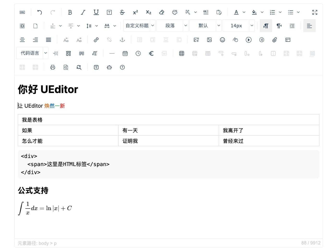
既然浏览器原生实现不可靠,开发者便开始在 contenteditable 之上构建封装层。CKEditor、TinyMCE、UEditor 等经典编辑器通过拦截 document.execCommand,用自己的命令系统替代浏览器默认行为,试图在混乱之上建立秩序。这一阶段的核心特征是:HTML 既是编辑器的内部状态,也是最终渲染结果。
然而,这种架构存在一个结构性矛盾:编辑器为了控制表现,不得不维护一套私有样式和 HTML 规范,但它又无法完全抛弃浏览器的渲染管线。HTML 与最终视觉呈现之间仍然隔着 CSS 解析、浏览器默认样式和平台差异的漫长路径。WYSIWYG(所见即所得)在此变成了一种近似幻觉——用户在编辑器中看到的,与邮件客户端、移动端或打印预览中看到的,往往并非同一回事。
对 HTML 路径的失望,催生了一场更为激进的叛逃。Google Docs 的新版编辑器彻底放弃了 contenteditable 和 DOM,转而基于 Canvas 自绘整个编辑界面:自己管理光标、自己实现文本布局、甚至自己解析字体 。腾讯文档、WPS Web 版也走上了类似的道路,无论是否使用 Canvas,核心思路都是独立实现编辑与排版功能,将浏览器降级为一块像素画布。
这种 L2 级编辑器的优势显而易见:跨平台一致性、精确的像素级控制、协作编辑的自然支持。但它的代价同样高昂——如此重度的工程投入,只能由巨头维持,核心技术几乎不可能开源。这标志着编辑器架构的第一次根本性分离:文档模型与渲染视图彻底解耦。编辑操作不再直接修改 HTML,而是修改一个抽象的数据结构,再由自绘引擎将其映射为像素。
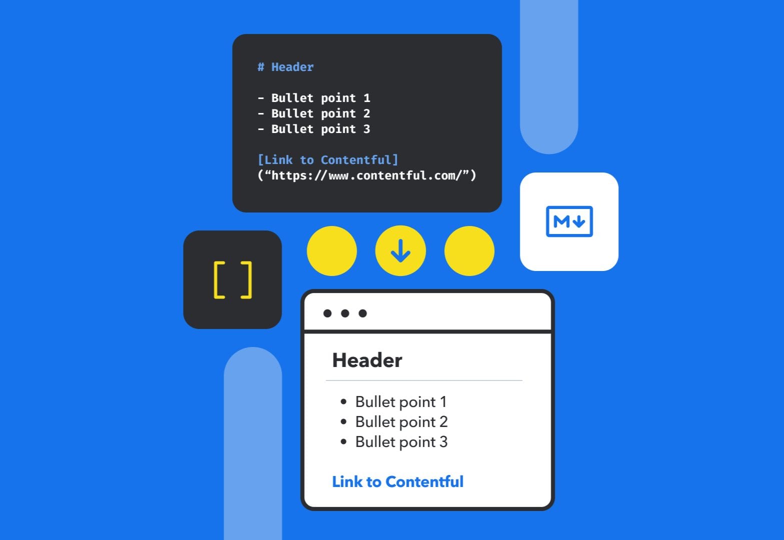
当 Canvas 自绘走向封闭的重工程时,另一条路径选择了截然相反的方向:极度简化。Markdown 的流行并非因为它强大,而是因为它有意识地放弃能力以换取一致性。CommonMark 和后来的 GitHub Flavored Markdown (GFM) 定义了一个最小可用的语法子集,使得后端渲染变得 trivial,任何文本编辑器都能成为 Markdown 的 WYSIWYG 前端。
然而,这种极简很快遇到了边界。插入媒体、复杂排版、交互组件——这些需求超出了 Markdown 的设计初衷。社区开始扩展语法,但方言的碎片化又削弱了“通用格式”的核心价值。Asciidoc、reStructuredText、MediaWiki 等替代方案在特定领域(技术文档、百科)取得成功,但没有一个能覆盖全部场景。Markdown 证明了轻量标记语言的价值,也暴露了它们的 ceiling。
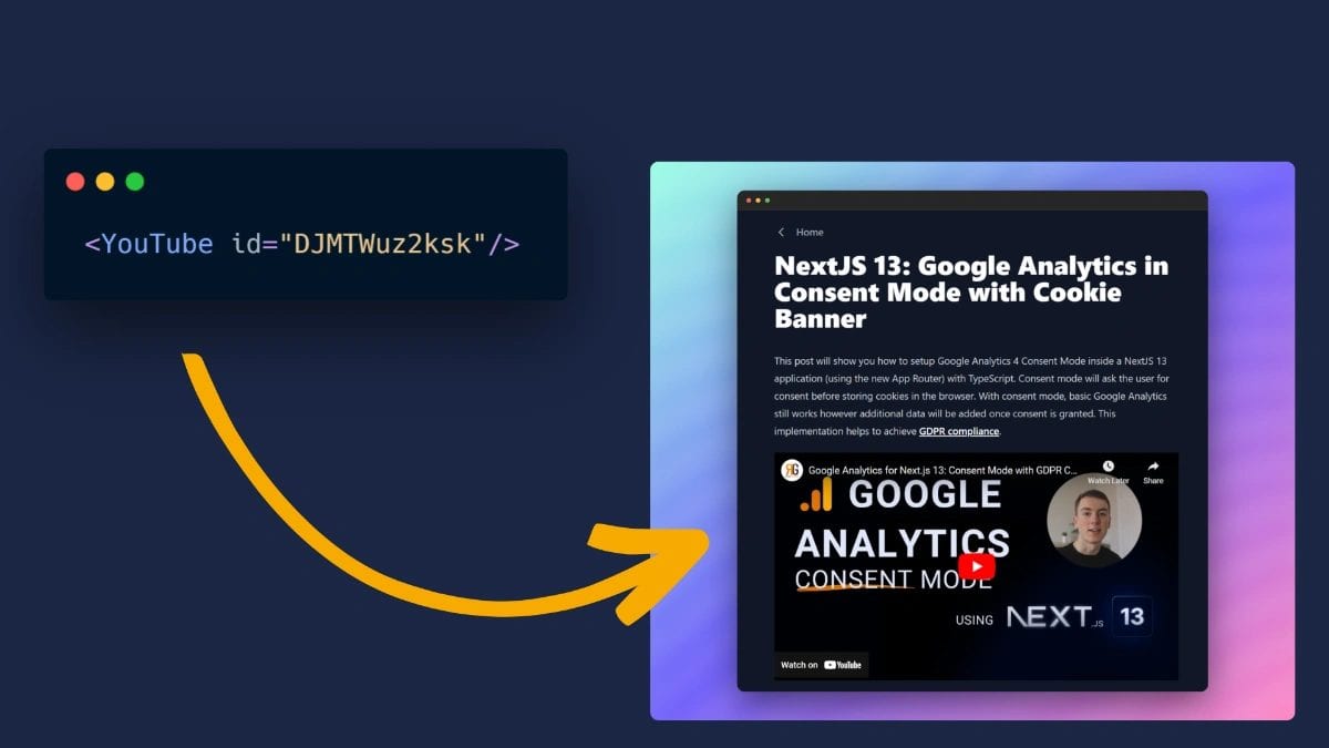
面对 Markdown 的表达能力瓶颈,社区探索出两条路径:降级回 HTML,或扩展标记语法。Hexo 的标签插件,都是在不破坏 Markdown 纯文本观感的前提下注入元数据。而 MDX 则走得更激进:它将 JSX 组件直接嵌入 Markdown,让 Markdown 从“标记语言”进化为“内容编程语言”。
MDX 的演进本身就充满启示。根据 John Otander 的回忆,MDX 最初的设计思路是“Markdown in JSX”——在 React 组件中通过模板字符串嵌入 Markdown。但很快发现,内容应该是第一公民,而非 JSX 的附庸。于是范式翻转,最终确立为“JSX in Markdown”,并通过 Babel 插件和 Webpack loader 在编译期完成转换,避免了运行时依赖 。MDX 在技术文档和组件库文档场景中取得了巨大成功,但它本质上是开发者的内容格式,依赖完整的 JS 运行时才能渲染,这使其难以成为大众编辑器或跨系统交换的通用底层。
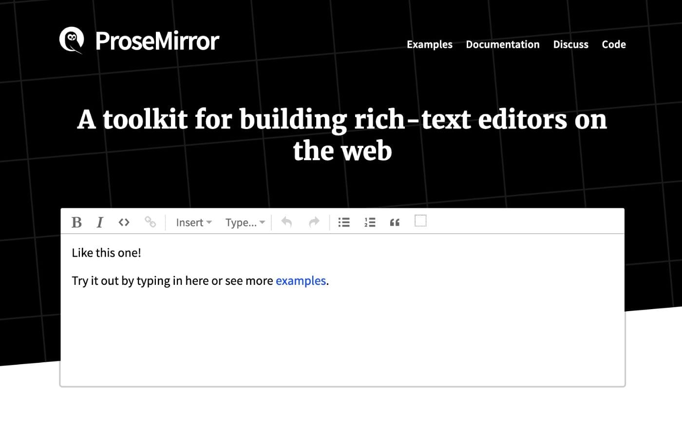
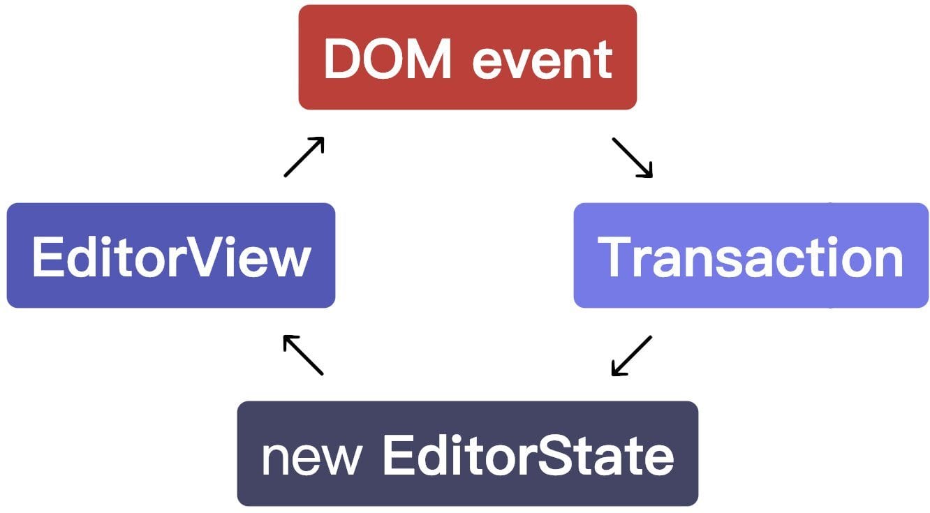
2015 年,Marijn Haverbeke——此前因 CodeMirror 名满天下的编辑器领域权威——开启了 ProseMirror 的众筹项目 。ProseMirror 的划时代意义在于,它首次系统性地提出了 Schema + Transform + Plugin 的三位一体架构:编辑器的状态是一个可序列化的 JSON 文档树,而非 HTML;所有编辑操作都是对 JSON 数据结构的纯函数变换;视图层只是这一模型的投影。
几乎与此同时,2016 年 Ian Storm Taylor 开源了 Slate.js,其核心理念与 ProseMirror 遥相呼应:Slate 的核心是一个“无预设 Schema”的纯 JSON 嵌套树模型,文档、选区、命令都围绕这一数据结构运作 。Slate 的文档模型极其简洁—EditorBlockInlineTextMark 五类节点构成全部世界,而序列化后的 JSON 完全可预测、可人工阅读 。
这一阶段标志着编辑器范式的彻底转向:HTML 不再是真相来源,它只是 JSON 模型的一种可能的渲染输出。ProseMirror 和 Slate 证明,编辑器的状态应该是一个与渲染无关的纯数据结构,而 HTML、Markdown、PDF 都只是这一模型的不同序列化视图。
JSON 文档模型的流行,与实时协作技术的成熟是同一枚硬币的两面。早期的协作编辑依赖 OT(Operational Transformation),但在 HTML 树或字符串上实现正确的 OT 算法极其复杂,边界情况极易导致状态不一致。
CRDT(Conflict-free Replicated Data Type)的崛起改变了这一局面。Yjs 作为当前最主流的 CRDT 库,采用 YATA 算法和二进制增量编码,能够高效处理文本编辑场景中的并发冲突 。更重要的是,Yjs 与 ProseMirror 的集成(通过 y-prosemirror 绑定)已经高度成熟:ProseMirror 的每一次 Transaction 被自动转换为 Yjs 的 CRDT 操作,网络层由 Hocuspocus 或 WebSocket provider 处理,开发者几乎无需关心冲突合并的细节 。
JSON/Block 模型之所以特别适合 CRDT,是因为树状结构天然支持按节点隔离冲突域。Notion 的块级模型(每个 Block 是一个独立节点)正是这一思路的极致体现——当两个用户同时编辑不同 Block 时,冲突解决是平凡的;即使在同一文本块内,Yjs 的 Y.Text 也能保证最终一致性。可以说,没有 JSON 文档模型的先声,现代 Web 协作编辑的民主化就不会发生。
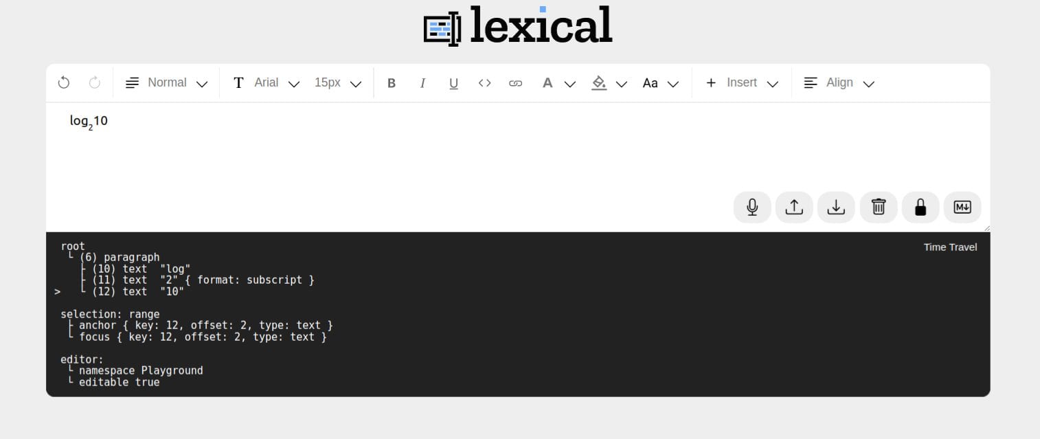
2022 年 4 月,Meta 开源了 Lexical,一个被定位为 Draft.js 继任者的可扩展文本编辑器框架 。Draft.js 曾基于 Immutable.js 为 Facebook 的笔记、评论和 Messenger 提供支持,但长期陷入维护模式,官方明确推荐用户迁移至 Lexical 。
Lexical 的设计哲学反映了 Meta 在超大规模场景下的经验:核心引擎仅 22kb(min+gzip),采用不可变状态树和事务批处理更新,与 React 的渲染模型深度对齐 。它通过插件系统按需加载功能——列表、链接、表格、Markdown 都是独立包,开发者只为自己使用的功能付费。在架构上,Lexical 同样遵循“模型优先”原则:它附着在 contentEditable 元素上,但开发者极少直接操作 DOM,而是通过声明式 API 与 Lexical 的编辑器状态交互 。
Lexical 的出现,加上基于 ProseMirror 的 Tiptap、BlockNote 等封装库的成熟,意味着结构化 Block 编辑器已经从 Notion 的闭源黑箱,变成了可复用的开源基础设施。这是 JSON 文档模型范式的最终胜利——它不再是先锋实验,而是行业标准。
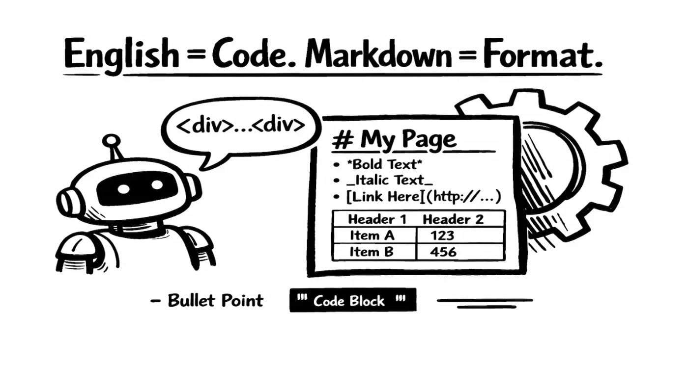
然而,就在 JSON Block 编辑器似乎要一统江湖之际,AI 大模型的爆发意外地将 Markdown 重新推上了王座。今天的 LLM 应用——从 ChatGPT 的 Canvas 到各类 RAG 系统——几乎无一例外地使用 Markdown 作为默认输出格式。
这种回潮有其结构性原因。首先,Markdown 的语法密度低,在 LLM 的上下文窗口中信息熵更高;其次,互联网的高质量训练语料(GitHub、StackOverflow、技术文档)本身就是 Markdown 为主,模型对其语法结构的先验知识更强;第三,Markdown 的双向可逆性——人类可以直接编辑模型生成的 Markdown,而无需理解复杂的 JSON 树结构。
但这也暴露了一个深刻的悖论:AI 需要 Markdown 的简洁,但用户需要 Block 编辑器的表达能力。当前的工程实践正在用“混合模型”弥合这一裂缝——底层存储和协作仍然基于 JSON/CRDT,但 AI 交互层使用 Markdown 作为“协议语言”,再由编辑器解析为 Block 结构。Notion AI、Obsidian 的 AI 插件,乃至各类 LLM 写作工具,都在采用这种双层架构。
从 contenteditable 的混沌,到 HTML 封装的挣扎,从 Canvas 自绘的封闭,到 Markdown 的极简,再到 JSON 模型的结构化和 AI 时代 Markdown 的意外回潮——这条曲线并非线性进步,而是一次次关于“谁掌握控制权”的螺旋上升。
Marijn Haverbeke 在 2015 年 salvage contentEditable 时,大概不会想到九年后 AI 会成为编辑器的核心用户之一;Meta 开源 Lexical 时,也未必预料到 Markdown 会在 LLM 语境下重新成为通用语。但贯穿始终的主线是清晰的:编辑器的状态必须是一个与渲染无关的、可序列化的、机器与人都能理解的数据结构。
谁能在 JSON 的结构性、Markdown 的文本友好性和 AI 的生成需求之间架起最优雅的桥梁,谁就能定义下一个十年的编辑器范式。这场演进,还远未终结。
2026-05-06 23:44:00

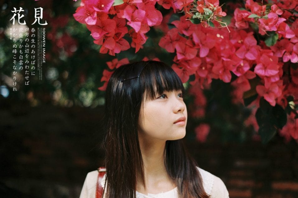
三角梅与花影的缘起,该从哪一页慢慢读起。风将盛夏的讯息叠入瓣间,夏至未至,满墙花色已先染红三分。午后暖阳像一位沉静的读者,缓缓翻阅夏日滚烫的序章,连流动的空气,都被烘得温柔微暖。

不过抬首低眉的一瞬,花影悄然落于腕间。像半句羞怯收口的私语,被清风轻系在脉搏之上。从此心跳有了温柔形状,随血脉起落沉浮,仿佛整个初夏的韵律,都妥帖藏在这一寸肌肤之下。

忍不住对着满墙繁花,低声倾诉心底藏事。红砖藤蔓静静听着,将心事悄悄卷进幽深砖缝。那些未曾出口的歌谣、未曾寄出的信笺,都在此处寻得归处,只待来年夏日重来,再逐一轻轻拆封。

心境忽然变得微妙难言。头顶紫红繁花汹涌盛放,宛如被整个初夏从身后温柔相拥,又在来不及回应时缓缓松开。只留一缕花香沾在裙角,在风里轻轻荡漾,化作一声欲言又止的轻叹,久久萦绕不散。
眼底忽然漫起温柔温度。仰望次第舒展的花瓣,恰似一场提前绽放的烟火,在夏至未至的晴空里静静燃烧。花枝拔节舒展,细碎光斑散落眉睫,仿佛有人把星子碾碎,轻轻敷在眼眸深处。

夏意在街巷两旁悄然拔节。离开繁花满墙的角落,浓荫将白衣染作浅绿,恰似一张缓缓显影的胶片。所有温柔都隐于暗影之中,静待某个慵懒午后、某双温柔眼眸,将光影定格成此生抹不去的回忆。
清风在身后静静伫立,像一位不忍惊扰的旁观者。手扶斑驳老墙,指尖抚过岁月刻下的纹路,砖缝青苔是沉默的乐谱,藏着世间未曾唱尽的温柔旋律。只待风起,只待人来,便轻声低吟,从头再叙一遍旧事。

人与盛夏,一同慢慢归于沉静。垂首时,身影落于裙边,如一阕降了声调的小夜曲,在地面缓缓流淌;闭目时,暖阳轻落眉心,似温热指尖轻轻按下一个和弦,力道不重,却足以撩动整颗心的震颤。
脚步在夏日里越走越缓。衣袂裙摆,鞋尖剪影,都在长路上写满流连不舍。那些牵过与未曾牵过的手,皆是花影里虚握的清风。明明无从紧握,偏偏难以放下,只好任它从指缝溜走,凝成一道温柔绵长的心痕。
从花墙下缓步掠过,裙裾迎风绽开伶仃花影。发丝轻扬,几片三角梅随风飘落,终究停驻原地。像一场来不及道别的目送,目送一季盛夏远去,目送所有说出口与藏心底的情愫,慢慢淡出时光。

逝去的黄昏与未至的清晨,都在凝望的眼波里层层重叠。有些花色,未曾用心辨认;有些盛夏,未曾真正奔赴。只需静静伫立,便成了季节最温柔的注脚,写满浅浅遗憾,也盛满圆满清宁。
行于花影,步履愈发从容缓慢。转身回眸间,影子在路面写满未竟的诗行。那些尘封心底的旋律从未被放声吟唱,却在这个慵懒午后,被阳光轻轻弹拨,化作看得见的音符,落满肩头,覆满来时归路。

刹那间,世间似有清响与柔光共生。抬手遮挡渐盛的日光,指缝漏下斑驳光斑,像把完整的盛夏裁成细碎片段。每一缕光影落于肩头,都在轻声低语:夏至未至,而恰好,你已在此等候。原来所有漫长等待,只为这一刻心安确认。

时光忽然变得沉重又轻盈。这座城池从不轻易老去,静立岁月深处,收纳每一段无人珍藏的黄昏。墙角堆积的落花,是时光写给人间的细碎便签,字迹被清风慢慢冲淡,只剩温柔轮廓,留待后来人细细品读、慢慢共情。

行至路尾,蓦然回眸。目光化作一缕温柔弦音,从此岸绵延至花影摇曳的深处。夏至未至,三角梅仍在枝头轻声呢喃,像盛夏藏在心底未尽的私语,被清风一遍遍反复低吟。盼有人来听,又怕有心人听懂——怕一旦听懂,便此生再也走不出这一季温柔花影。
2026-04-17 20:31:16

我们从小到大的教育方式中,藏着一个不易察觉的“陷阱”。
从识字启蒙开始,我们便被训练着去挖掘文字背后的“深意”。一篇课文的中心思想,一句诗词的弦外之音,甚至一个词语的隐含寓意——我们被教导要层层剖析,步步登高,最终将平凡的文字抬升到崇高的高度。阅读理解有标准答案,作文立意要高远深刻,连造句都要体现“正确的价值观”。这种训练如此根深蒂固,以至于它悄然内化为我们的思维定式,伴随我们走过学生时代,步入成年世界。
然而,这种习惯一旦走出课堂,便常常变了味。
如今的网络世界里,这样的场景屡见不鲜:某人发了一句无关紧要的感慨,评论区便开始“深度解读”;一张普通的照片,能被分析出“微妙的心理暗示”;一段日常的分享,往往被引申出“不可告人的动机”。我们似乎患上了“意义强迫症”——看到任何信息,第一反应不是理解字面意思,而是下意识地深挖其背后的“真实含义”。
这种过度联想的代价是巨大的。
它制造了大量本不存在的矛盾。朋友间一句无心的玩笑,被过度解读为“话里有话”;同事一个寻常的举动,被层层剖析出“深层意图”。本来相安无事,想着想着便琢磨出事来了,给自己徒增无数烦恼与戾气。更可怕的是,这种臆测出来的“真相”,往往成为攻击他人的武器——“你这么说是何居心”“你这么做一定有目的”。一场场网络骂战、人际冲突,很多时候并非源于真实的矛盾,而是源于我们丰富的“想象力”。
当然,我并非主张放弃思考。审视与反思是珍贵的品质,对事物的深度理解更是智慧的体现。但凡事皆有度,过犹不及。不是所有的话语都需要解码,不是所有的事件都需要升华,不是所有的细节都值得反复咀嚼。就像不是每一朵云都藏着暴风雨的预兆,不是每一次沉默都意味着不满与抗议。
学会区分“有意义的深度”与“无意义的过度”,是一种难得的智慧。有些话,听其表面便好;有些事,观其表象足矣。给自己留一点“不琢磨”的空间,给他人留一点“被误解”的宽容,生活反而会轻松许多。
人生并非处处有深意。成年人的世界里,很多事情并没有那么多弯弯绕绕,很多人也并没有那么多机关算尽。与其耗费心力去猜测、去解读、去赋予意义,不如学会一种更高级的处世哲学——筛选。
你无法改变别人的表达方式,无法阻止世界的纷繁复杂,但你可以选择如何接收信息、如何回应世界。觉得舒服的关系,就好好珍惜;感到疲惫的解读,就适时放下;无谓的纷争,一笑而过便好。接受那些你能接受的,改变那些你能改变的,至于其余的,不如让它随风而去。
六祖慧能曾言:“菩提本无树,明镜亦非台。本来无一物,何处惹尘埃。”
心中若无过度解读的执念,眼前便少了许多无事生非的纷扰。放下那把总在挖掘的铲子,或许我们会发现:生活本身,比任何解读都更加简单,也更加美好。

2026-04-16 23:08:23
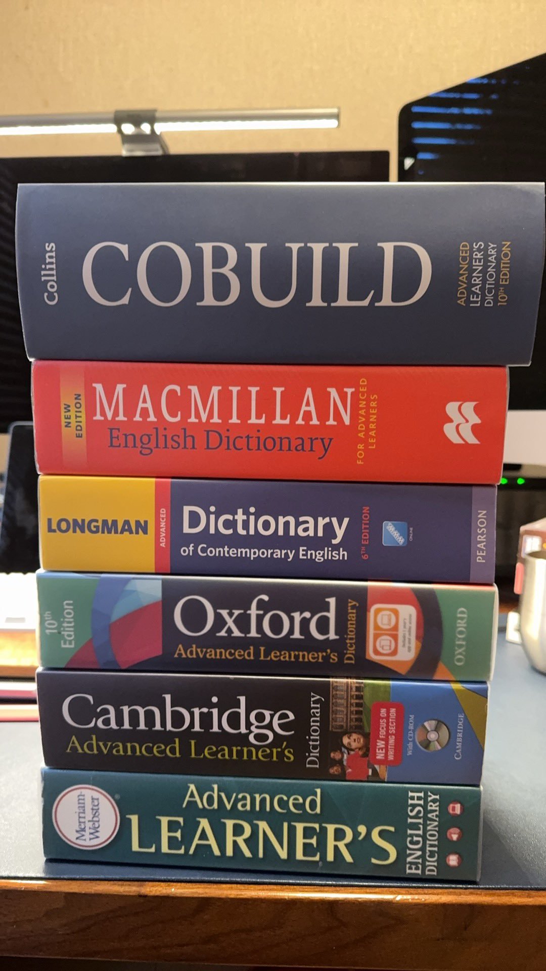
牛津高阶第 11 版出版已有三个多月,目前仅在印度本土印刷上架实体书,东非等部分地区也有发售,这与人们的传统认知并不相符。毕竟,中国才是全球最大的英语学习市场。
不过,国内主要引进的一直是英汉双解版本,外研社近十几年来也极少出版纯英英词典,近期仅推出了柯林斯第 9 版。更不必说,海笛、万邦等平台几乎垄断了国内的数字词典 APP 市场。
另一方面,除了在校不能使用手机的学生群体,纸质词典在查词效率上几乎没有任何优势。即便是卡西欧 Exword 这类老牌电子词典,也渐渐不敌「物書堂」等词典 APP。牛津官方 APP 更是收录了最新的权威数据,内置真人发音;若不想付费,iOS 端也有 OpenMDict 这类查词软件,可导入网友制作的各类免费词典资源。
手机词典还支持多词典同步检索对比、生词收藏、反向查阅等功能,这些都是纸质词典无法实现的,更不用说查词速度、新词收录与词频更新等方面的差距。
因此我十分理解,牛津高阶 11 版为何只在部分经济欠发达地区先行推出纸质版。或者说,习惯了 APP 查词的便捷后,很少有人还愿意回归纸质词典。
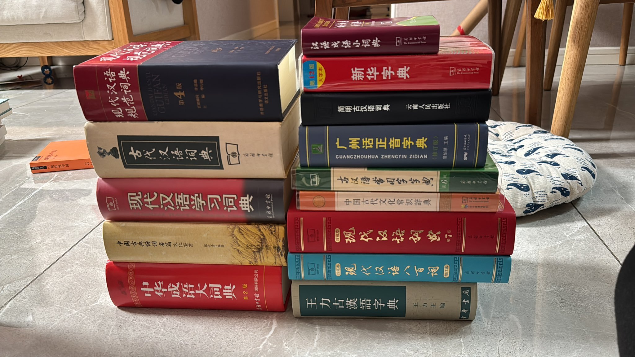
但作为一名 90 后,我始终难以割舍对纸质词典的情结。
人生中的第一本纸质词典,是从垃圾桶里捡回来的《现代汉语词典(增补本)》。它被初一同学撕烂了封皮,书侧也被涂得漆黑。我值日倒垃圾时发现,悄悄捡回宿舍,用胶带仔细粘好,视若珍宝。这本词典陪伴我直到高三毕业,时常翻阅,每个字、每个义项都至少看过两遍。
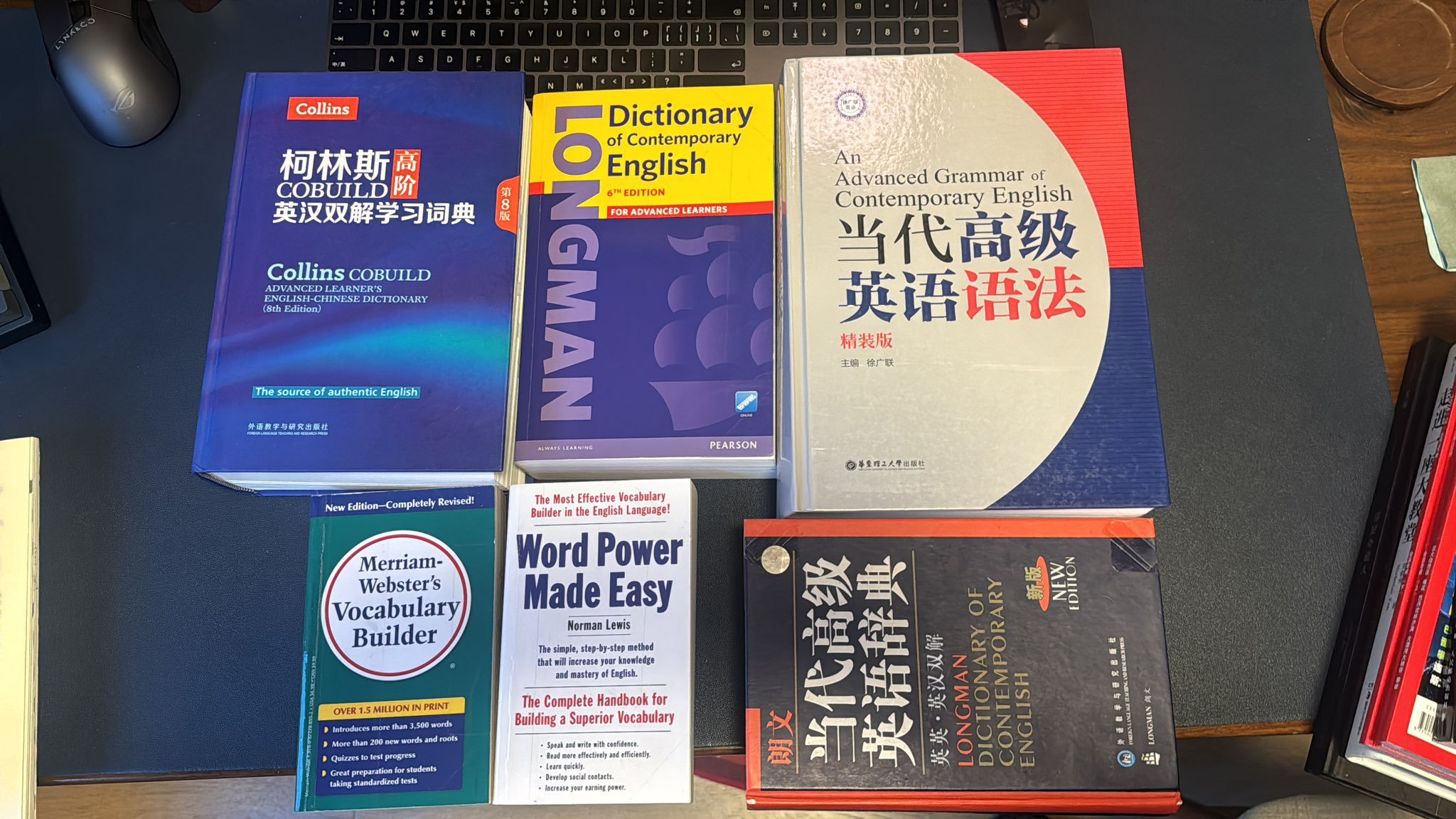
第二本则是《朗文当代高级英语辞典·英英英汉双解(修订版)》。彼时它的双解版权刚从商务印书馆转至外研社,因此封面沿用了商务版样式,内容以台湾商务国际的译本为底本,还标注了 KK 音标。这是我的第一本英语学习词典,感谢当时的老师,专门用一整节课教我们如何正确使用词典。那时每天坐在厦门环岛路的公交车上,我都在翻看背诵,至今仍能记起里面许多经典例句。
前文已说尽电子词典的种种优势,若非要讲清我放不下纸质词典的缘由,大概有这几点:
一是实体翻阅的沉浸感。人的记忆有时依托于类似记忆宫殿的立体感知,翻阅纸质词典时更易专注记忆、不受干扰,这一点与阅读实体书籍相通。
二是通读的满足感。至今我已通读过不下五本词典,这种体验是电子词典无法给予的。
三是偶然发现的惊喜。查阅纸质词典并非像电子词典那样目标明确,翻页过程中,偶然瞥见的新词、插图、学习小贴士,常常会让我停下脚步细细阅读。
我想,这些便是时至今日,我依然愿意入手一本实体词典的最大原因。
2026-04-15 21:10:33
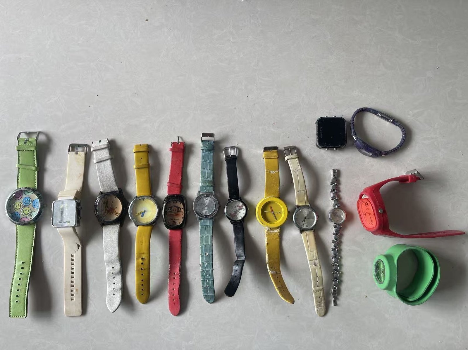

那是三月的一个午后,窗外梨花正盛,每一瓣都是春日投递的短笺。手机忽然一震,一张旧照从屏幕彼端浮上来:数枚女式旧表静静躺着,表带褪色斑驳,表盘形状各异,像一群被时光遗忘的细小生灵。
“中学时戴过的,”夫人在消息里附带了声轻笑,“母亲今日收拾阁楼翻了出来,问我还留不留,不留便扔了。”
我们相识于六年前的新岁。彼时经人引荐,微信上往来数旬,终得一见。那日海底捞灯火喧腾,人影如织,我于浮世喧嚣中一眼就望见了她。目光顺势垂落,恰好停在她左手腕间——那里栖着一片胎记,色如深墨,形似一枚表盘。
后来,当我们从恋人成为未婚夫妻,她曾动念入院,欲以医术消去那印记。前几日的某个深夜,闲谈间又说起此事,她只是淡淡地说:“习惯了,且留着吧。只要无虞,便是身体的一部分。”
故而那排旧表映入眼帘的刹那,我已了然于心。尚未开口询问,她的消息又至。
“那时为何总要戴着手表?只因腕间有这胎记,自觉丑陋,怕人侧目,便日日以表带遮掩。”
“其实除我之外,根本无人在意。只是年少时不懂得,直至踏入大学校门,方敢正视这片印记,摘下手表,让它重见天光。”
这番话像是忽然掀开了阁楼的另一角,那些被压在箱底的年少心事,一下子见了光。那些细微如尘的自卑——或是人前始终低垂的颈项,或是言语间游移的目光,或是盛夏里执意不肯褪下的长袖——此刻竟如尘埃般,在午后的光柱里纷纷扬扬。
想来世人皆携“胎记”而生。少年时,总自命为命运写废的草稿,于喧嚣人世中暴露着无法遮掩的瑕疵。于是拼命寻那遮饰之物:或是一件宽大的衫袍,或是一句故作清高的言语,或是一段刻意疏离的静默。我们以遮掩为铠甲,以为藏得足够深,便不会被世间看穿那色厉内荏的仓皇。
然而岁月终究会教给我们,那些曾以为会招来侧目的“不同”,不过是生命独有的纹理。正如古木不会因年轮而羞赧,江河不会因曲折而拒海。真正的成长,非是将胎记从肌肤上剜去,而是学会在日光下坦然展示那一片深色的印记,让它成为躯体叙事的一部分,而非需终生遮掩的秘密。
阁楼上那些旧表,终将被清理。如同我们终将告别那个在镜前反复审视自己的年纪。那些褪色的表带与斑驳的表盘,何尝不是另一种形式的茧——曾经紧紧束缚,却也在无形中丈量着一段从遮掩到坦然的距离。
窗外,梨花依旧似雪。而那个不再需要以手表遮掩时光的女子,早已在岁月的浸润中,长成了亭亭的模样。