2026-06-01 00:30:00
和 Debug 日志、SRE 日志一个系列,优化日志用来复盘一些可以公开的折腾经历。
这一篇的主角是 PicImpact——我自己在用的那个开源图床,跑在 photos.manjusaka.me 上,托管着我这几年拍的猫猫狗狗。去年年终总结里我写过一句「把自建图床项目的代码拾掇了很多」,这篇就算是那句话的注脚。前后断断续续修了一轮,修复点其实都不大,但中间冒出来的几个回归是真的有意思,尤其是最后那个 WebGL 的坑,我愿称之为本年度最佳。
日常用下来,对着隔壁 afilmory 抄作业,我把 PicImpact 的毛病列成了五条:
看着像五个独立的问题,真顺着查下去会发现,根子其实是同一个:这个图床在「该喂给浏览器什么」这件事上,从一开始就喂错了。
下面不按 PR 的顺序讲,按「病灶」讲。顺带一提,整个过程是拆成一堆子任务、各走各的 feature branch + PR 推进的,PR 都提给了上游 besscroft/PicImpact。
先说第五条,因为它是杠杆最长的一根撬棍——把它撬动了,③④ 也跟着松了大半。
原来的逻辑朴素得感人:缩略图走一张 preview,点开看大图,直接怼原图。问题是我那台 Z8 出的片子动辄 8256×5504、十几兆一张,首页一铺二三十张……移动端内存那点家底,就这么被噎死了。
正经做法是预处理出响应式变体:上传的时候把每张图压成一梯队不同宽度的 AVIF([320, 480, 640, …, 2560]),前端按 sizes 取对应那一档。这里有两个我觉得值得贴一下的细节。
第一,一张原图只解码一次。十几兆的图解码本身就不便宜,要是每个档位都从头解一遍,那预处理能慢到姥姥家:
1 |
// server/lib/image-variants.ts —— 解码 + EXIF 纠正只做一次,8 个档位都从 clone 出来 |
AVIF 的 effort 我从默认的 4 压到了 2,编码快了两倍多(约 2.6 倍),体积基本没差别,属于白捡的。
第二,变体的 key 用原图的 sha256 来做内容寻址。这样内容一变 key 就变,配上 Cache-Control: immutable 就能永久缓存,压根不用操心失效这事:
1 |
const digest = createHash('sha256').update(input).digest('hex').slice(0, 32) |
剩下就是让前端真的去吃这些变体。这里有个一定要注意的坑:next/image 默认会把图片全绕回 Node 服务器去做优化(/_next/image),那我 CDN 不就白搭了么。所以得写个自定义 loader 直接拼 CDN 上的 URL:
1 |
// lib/image/loader.ts |
存量那一千来张(实测 1091 张)用一个基于 PG 的任务队列慢慢 backfill 补齐。期间还踩了个小坑:有几张 11008×16512、182MP 的全景,把我们自己设的 100MP 解压上限给顶爆了——那个上限当初是为了防解压炸弹,比 sharp 默认的约 268MP 还严,于是单独给放宽到了 500MP。
效果是相当离谱的。同一张图(DSC_7956,原图 18.08MB):
原图 JPG:18.08 MB
旧的 preview(webp):164 KB
网格用的 AVIF 640:5.19 KB,约 3480 倍
灯箱用的 AVIF 2560:24.1 KB
一个首页 24 张图,从「原图加起来 400 多兆」变成「一百多 KB」。后面做 trace 的时候我看到首屏那张 LCP 图的下载耗时是 89 微秒——微秒。⑤ 和大半个 ④ 就这么没了。
这里有条原则我从头贯彻到尾:网格和默认详情页永远不碰原图,原图只有一个地方会加载,就是用户主动点开全屏缩放的时候。记住这个「例外」,它后面要出大事。
字节数搞定,剩下是「怎么把它们画出来」。
瀑布流原来是 CSS 多列(columns-*),这玩意有个阴间的地方:每翻一页追加新图,整个累积的 DOM 会重新挂载、重排,把前面所有图的位置全打乱重来一遍。换成 masonic 做窗口化虚拟瀑布流之后,item 只测一次、绝对定位、只挂视口里那些,滚动顺了不止一个档次。
移动端那个无限崩溃循环(③)最唬人,根子在无限滚动的 IntersectionObserver——回调闭包把过期的 state 给捕获了,于是某些时序下它会发了疯一样地「加载下一页」,移动端就这么被拖崩、刷新、再崩。把状态收敛进 ref、再把预加载的 rootMargin 拉到约 1.5 个视口(变体那么小,预加载激进点完全不亏),滚到底再也不用干等接口了。
动画那块(①)就是常规操作:合理用 will-change、blurhash 占位 + 宽高比盒子防止图片加载时的布局回流。后者顺手把 CLS 摁到了 0.01。
在途的 PR 合完,我对线上做了一轮 trace + Lighthouse。头号发现是 LCP 4.69s,差评。
但拆开一看就很有意思:那张 LCP 图自己 89 微秒就下完了,慢全慢在「发现」上——2.77s 的 load delay。三项 LCP discovery 检查全军覆没:没 fetchpriority=high、用了 loading=lazy、而且压根不在初始 HTML 里。
最后这条是命门:画廊是 dynamic(ssr: false) 的纯客户端组件,首图根本不在服务端吐的 HTML 里,浏览器的 preload scanner 自然发现不了,得等 hydration + 动态 import 跑完才开始发请求。
修法就是把首图捞回初始 HTML:首屏头几张标 priority,再在服务端往 <head> 里塞一条响应式的 AVIF preload-link。imagesrcset 直接复用前面那套档梯常量生成、并且复刻了 next/image 自己的 getWidths 选档逻辑,保证 scanner 和真正的 <img> 选到的是同一个候选——不会重复下两次。
TTFB 那 700 来毫秒也没放过。页面是每次请求都打 DB 的动态渲染,在公开只读的那些数据函数上包一层 unstable_cache + tag 失效(只缓存全局公开数据,鉴权的一概不碰,写操作触发失效避免上传后长期 stale),TTFB 降了约 38%(/lotus 实测从 ~0.65s 到 ~0.40s)。
再把瀑布流容器那个 role="grid" 改成 role="list"(grid 要求子节点是 row/gridcell,我这一堆链接挂在 grid 底下本来就是 ARIA 契约违例),移动端 a11y 从 90 干到了 100。
一轮下来:LCP 4.69s → 2.46s,CLS 0.01,a11y 满分,TTFB 砍掉小四成。本以为可以收工了——然后就开始还债了。
性能优化这事最迷人的地方就在于,你每堵上一个窟窿,新的窟窿就从你没盯着的地方冒出来。
第一个,详情页退出来之后,整个相册从 AVIF 退化回了原图/webp。查下来是变体的 CDN base(variantBaseUrl)走的是客户端 SWR 拿的配置,软导航(详情→返回)让画廊重新挂载的那一瞬间,配置还没回来、base 是空的,整个变体阶梯就失效了。给那个 SWR hook 加一层模块级的 fallbackData 兜住上次的值就好。先记住这个「配置异步到达的缝隙」,它马上还要再咬我一口。
第二个,移动端崩溃循环——它回来了。现象是加载相册时 network 里会请求一大堆「明明已经优化掉的」preview。devtools 一抓,硬刷一次 /dog:40 张 AVIF + 24 张 preview,64 个请求,而且这个数字 7.5 秒内纹丝不动,说明不是死循环,是一次性的双重加载。
根子还是那条缝隙。冷加载第一帧 variantBaseUrl 是空的,于是:
1 |
// masonry-photo-item.tsx:base 为空 → hasReadyVariants 为 false → 回落去拉 preview |
先 preview 后 AVIF,白下一轮。桌面顶多浪费点流量,移动端是 24 张 preview 的解码内存峰值直接把页面顶 OOM,崩了刷、刷了崩。修法是釜底抽薪:页面本来就是 server component,服务端 resolve 出 variantBaseUrl 之后当 prop 直接透传给画廊,第一帧就有 base,焊死这条缝。
第三个最精彩,是个 React 和 WebGL 凑一块儿才能凑出来的坑。现象很具体:详情页点图进缩放(一个 WebGL viewer),第一次好好的,关掉之前再点第二次,整个页面当场去世,图也没了。
老规矩,先 devtools 复现,给 WebGL context 的创建/丢失打点:
第一次开:context 活着 ✓
关闭:context lost = 1
第二次开:没有新建 context,而且isContextLost() = true
顺着这条线索捋,根因是这么一串:
这个 viewer 是用 React 的 <Activity mode="hidden/visible"> 来显隐的。<Activity> 有个很要命的语义——隐藏的时候它会跑子组件的 effect cleanup,但保留 DOM(同一个 <canvas>)和 state。而我之前为了修「相册→详情→缩放反复进出会泄漏 WebGL context」(浏览器活跃 context 大概 16 个就到顶了),在 viewer 的 cleanup 里加了一刀 destroy:
1 |
// WebGLImageViewer.tsx —— 这个 cleanup,在 Activity 隐藏时也会跑 |
于是关闭 modal(Activity 隐藏)的时候,这个 cleanup 跑了,loseContext() 把那块被 Activity 留着复用的 canvas 的 context 永久弄丢了。等第二次打开,effect 重新跑,可 isInitialized 这个 state 又被 Activity 原样保留着——初始化函数里那句 if (isInitialized) return 的守卫,要么短路(不重建引擎,于是留你对着一块死 canvas 发呆,图不显示),要么没短路(试图在死 context 上重建,createProgram() 返回 null,下一行 attachShader(null, …) 直接抛异常,整页带走)。同一个 bug 两种死法,全看那个守卫这次短没短路,挺哲学的。
说白了就是:我把 destroy 绑错了地方,绑在了「关闭缩放」上,可它本该只在「离开详情页」的时候触发。
第一版修法(#509)图省事,直接把 viewer 从 <Activity> 显隐改成条件挂载/卸载。崩是不崩了,可很快就回过味来——这版 UX 反而退化了:每次开都重建引擎、重新解码原图,缩放和平移的状态也全丢了。原来那套设计是能在 modal 里复用同一个 context、把缩放状态留着的,这才是好体验。
最终版(#510)想明白了:viewer 首次打开之后就一直挂着别卸,开关只用 CSS visibility 切:
1 |
{hasOpenedFullScreen && ( |
不卸载就不跑 cleanup,同一个 context 跨开关复用,缩放状态稳稳留着,也不崩;而 destroy 只在 ProgressiveImage 真正卸载(离开详情页)的时候才触发,防泄漏那一刀的收益原样保留。
这里还有个细节:用 visibility:hidden 而不是 display:none。后者会把 canvas 尺寸变成 0×0,引擎算 fit-to-screen 的 scale 时会被 clamp 成 1,重新显示的时候就把你的缩放给重置了。visibility:hidden 保住尺寸,绕开这条路。
React <Activity> 那套「隐藏 == 卸 effect,但 state 和 DOM 都留着」的语义,碰上「持有原生资源」的组件,是真的隐蔽。
回头看,⑤ 那一刀(原图体积)是性价比最高的——图床这东西,先把「喂给浏览器什么」搞对,一多半的毛病会自己消停。剩下的,与其说是优化,不如说是在「修好主问题之后,挨个去还它牵出来的债」:退化、双载、Activity 的生命周期,没一个是一开始就看得见的。
要说有什么方法论,大概就一条:能 devtools / curl / Lighthouse 量出来的,就别猜。尤其 debug,先稳定复现、揪到根因再动手,比「改改这个看看?」要快得多。
图床现在用着是真舒服了。下次再翻小熊和小狗的照片,至少不用再等那一下卡顿。
一万年太长,我们只优化今朝(
收工。
2026-03-23 22:30:00
最近给一个后端服务做 perf,跑了一发 py-spy 出来火焰图,盯着看了一会儿,发现 pydantic.main.__init__ 这一条在主热路径上占了一个让人挺难绷的比例。做了几轮调整之后顺手把这件事记一下——核心想说的是:对一个 web 服务来说,数据校验从来不是免费的,pydantic 也一样。它有它的边界,越界使用就要付出对应的代价。
某个内部业务服务,写法上挺标准——FastAPI + uvicorn + pydantic + psycopg,业务里所有”长得像数据”的东西,从 DB 行、内部传递的中间态、到 API response,全部都用 BaseModel 表达。看起来一致、规整,review 起来也舒服。
直到我们因为 P95 不太好看,跑了一发 py-spy:
1 |
py-spy record --duration 60 --rate 100 --output flame.svg --pid <uvicorn-worker-pid> |
火焰图大约 8,700 个采样点,里面让我多看了一眼的是:
pydantic/main.py:250 也就是 BaseModel.__init__,单条最厚的火焰柱占了 22.65%(约 1,982 samples)__init__ 路径又占了 6.81%最骚的是,这些 __init__ 大部分根本不是用户请求的入口校验,而是从我们自己的 PostgreSQL 里 SELECT 出来的行,被 psycopg.rows.class_row(SomeModel) 一行一行喂给 BaseModel.__init__ 的——也就是说,我们在拿”自己写进去的、Schema 完全可控的数据”,反复跑一套带 schema validation 的实例化流程。
那一刻就一个念头:这事真不值得。
Pydantic v2 已经把 validator 内核换成 Rust 写的 pydantic-core 了,比 v1 快了一个数量级。所以很多人下意识会觉得 “v2 的开销可以忽略”。这个印象大致没错——但只要你的 QPS 再高一点、单次请求里要构造的对象再多一点,”忽略不计的开销” × N 之后,它会非常明确地出现在你的 flame graph 上。
更重要的是,pydantic v2 快的是 校验本身。但你每实例化一次 BaseModel,整条链路是这样的:
1 |
__init__ 入口 |
哪怕你的 model 没有任何 validator、没有任何 Field(...),进 rust 转一圈再回来这件事本身就有不可压缩的成本——函数调用、字典构造、属性写入,每一项都要钱。
而把这套机制用在 从可信源反序列化 的场景上,大部分钱花得没意义——你这一行就是你刚才 INSERT 进去的,schema 对不上的概率约等于”你的 migration 没跑过”,那已经是另一类问题了。
把日常项目里 BaseModel 出现的地方分一下类,差不多是这五种:
pydantic-settings 读 YAML / env,启动时一次性校验field_validator / model_validator 的领域对象,比如 “金额必须是正数、组合字段必须满足某个不变式”前四个有明确收益——schema 是契约,validation 就是这份契约的执行机制,它的运行时开销换的是 类型/不变式上的安全保证。
第五个,几乎全是白送的开销。这一类对象是在你自己写的代码里产生、在你自己写的代码里消费的,schema 已经被静态类型检查器(mypy / ty)和 beartype 之类工具覆盖到了;运行时再跑一次 pydantic 的校验,校验的对象要么是你 5 行前刚 query 出来的,要么是你 3 行前刚自己 Item(...) 构造的。换句话说,你是在校验你自己。
那第五类该用什么?答案非常无聊——标准库的 @dataclass,加 slots=True:
1 |
from dataclasses import dataclass |
slots=True 让实例不再有 __dict__,每次构造省一份哈希表分配,访问字段也直接走 C 层 slot。配合 beartype 的运行时类型检查(如果你像我们一样在 __init__.py 里 beartype_this_package()),整体的”类型安全度”和你用 pydantic 是同一个量级的,但开销低得多。
更顺的一点是:psycopg 的 class_row 原生支持 dataclass,几乎是无缝替换:
1 |
from psycopg.rows import class_row |
调用侧的体感和原来一模一样——你照样有 .id、.value、.position,照样能被 ty / mypy 检查类型,照样能 for item in items: ...。差别只是火焰图里那条粗柱子掉下去了。
把上面的话翻成代码。假设我们要做一个 /items 接口,从 DB 取数据、做点轻量计算、然后返给调用方:
1 |
from dataclasses import dataclass |
整段代码里 pydantic 只活在两个位置:进来的请求 和 出去的响应。中间所有”只在我们自己代码里活动”的对象,全是 dataclass。这是一种很朴素的边界感——pydantic 守门,dataclass 干活。
不是所有看起来”内部”的 model 都该被改成 dataclass。下面这些情况,老老实实留着 pydantic:
field_validator / model_validator)—— 这些校验本身就是业务规则的载体model_dump() / model_dump_json() 做序列化 —— pydantic 的 dump 比手写转换更稳model_validate() / TypeAdapter 做反序列化 —— 输入来源不可信ConfigDict 配字段别名、from_attributes 之类的特性BaseModel 且子类依赖父类的 schema 推导pydantic-settings)—— 启动时一次性校验,是非常划算的开销辨认起来其实很机械——把这个 model 类的整个引用图扫一遍,看它有没有上面这些特性或这些用法。没有任何一条命中的,那它就是一个伪装成 model 的 NamedTuple,可以下放到 dataclass。
每次新加一个数据结构时,先按下面这串问题走一遍:
1 |
要加一个新的 data class |
这套规则不是要”消灭 pydantic”,而是把它放回它该在的地方——校验和序列化。其他位置上,标准库 + 类型检查器已经能给你足够的安全感,没必要额外缴一份运行时校验税。
回到那个火焰图。把”纯数据容器”那一类换成 @dataclass(slots=True) 之后,再跑了一次同等压力的 profile,主热路径上 pydantic.main.__init__ 的占比从 20%+ 掉到了零点几个百分点,相同 QPS 下 P95 也跟着下来一截。代码量倒没什么变化,受影响的也就是十来个类——但收益挺真实。
写到这里其实想说的话已经讲完了:
数据校验这件事,从来不是越多越好。它有明确的边界——边界之内是契约和安全,边界之外是无谓的开销。Pydantic 是非常好的工具,但用它的人也得知道自己什么时候用、为什么用。
下次起新项目,先想清楚这条边界画在哪。等到 flame graph 上 pydantic.main.__init__ 已经长成一根粗柱子才回过头来想,其实就晚了一步——好在还来得及。
差不多就这样。
2026-03-15 22:00:00
过去这一年我们团队陆陆续续做了几个 AI Service——大多是拿 FastAPI 包一个模型,再对外出 API。做到第三四个的时候我意识到一个尴尬的事实:每个项目长得都差不多,但每次起新项目还是在从零开始复制粘贴,而且不同的人写出来的目录结构、配置方式、metrics 命名都不太一样。一个新人接手第二个服务的时候,几乎要把第一个服务的认知全部重学一遍。
这篇文章想聊的不是某个具体框架,而是把这几个项目踩过的坑、迭代下来的设计、留下来的规范集中讲一遍——也算是给”维护一个模型 API 服务”这件事做一次复盘。
把”维护一个模型 API 服务”拆开看,其实是几个相互独立但又互相影响的小问题:项目长什么样、配置怎么分层、模型版本怎么迭代、可观测性怎么做、日常开发流程怎么走、CI 和镜像怎么发。下面按这几个维度逐个聊。
先看目录结构。我们最终收敛到的样子是:
1 |
src/<service_name>/ |
跟我们最早的版本比,最大的变化是引入了版本子目录。顶层的 handler.py 退化成了抽象基类,每个版本(v1、v2……)有自己的 handler 和 router。这是某个项目从 v1 演进到 v2 的时候被迫定型下来的——你不可能在原地修改老接口,又要让两个模型同时在线,唯一可行的就是物理隔离。
下面挑几个真正影响维护体验的点展开聊。
每个包的 __init__.py 第一行:
1 |
from beartype.claw import beartype_this_package |
beartype_this_package() 会给整个包的所有函数挂上运行时类型检查,开销接近零。它能抓住静态检查器搞不定的那一类 bug——你函数签名写的是 str,但运行时传进来一个 None;或者 tensor shape 不对;或者某个第三方库返回值的类型和文档不一致。
在 AI Service 这种场景里,模型推理链路上的类型错误特别常见——预处理、tokenize、forward、后处理,每一步都可能有数据形状或类型上的微妙差异。能在 import 时就把网撒开,越早暴露越好。
这是看起来朴素但实战非常关键的一个设计——我们把配置严格分成三类:
代码层面 Secret 和 App 是两个独立的 pydantic-settings 类:
1 |
class SecretSettings(BaseSettings): |
这种分层一开始看起来啰嗦,但维护几个项目下来你会发现:每次出”配置爆炸”问题、每次部署混乱,几乎都来自把这三类东西混在一起处理。强制分层之后,K8s 的 Secret、ConfigMap、Deployment args 各管各的,review 起来一目了然。
整个项目最值得说的一个设计决策——用注册表 + 动态导入来管理多版本,让 app.py 在加新版本时一行不用改。
app.py 里有两个 registry dict:
1 |
ROUTER_REGISTRY: dict[str, str] = { |
create_app 接受一个版本列表,支持同时跑多个版本:
1 |
def create_app(api_versions: list[str] | None = None) -> FastAPI: |
lifespan 遍历版本列表,动态加载每个版本的 Handler,存到不同的 app.state 属性上:
1 |
|
这个设计的好处是:app.py 不需要 import 任何具体版本的模块,加新版本就是加文件 + 加 registry 条目。换句话说,核心入口对版本扩展是封闭的,对版本添加是开放的——OCP 在这种场景下特别好用。
顶层 handler.py 定义 BaseHandler ABC 和共享的 schema:
1 |
class BaseHandler(ABC): |
每个版本的 handler.py 实现具体的模型加载,并提供一个 get_handler 读取自己那个 app.state 属性:
1 |
# v1/handler.py |
每个版本的 router.py 用 register_router(app) 闭包模式定义路由:
1 |
# v1/router.py — v1 没有前缀(默认版本) |
注意 v1 的路由没有前缀(路径就是 /predict),v2 才开始加 /v2 前缀。这是对历史的一种妥协——v1 是最早的版本,改路径会破坏已有消费者,所以新增版本的代价由新版本自己承担。
所有 CPU 密集的推理操作都用 asyncio.to_thread 包起来。路由函数的返回值类型注解就是响应模型——不用 response_model= 参数,直接写 -> list[PredictResponse],FastAPI 会自动推断。
讲完结构,最容易踩坑的部分是模型版本迭代。我们给自己立了一条铁律:
NEVER modify or rename an existing API route when adding a new model version.
听起来是废话,但真做的时候很多人会犯错。以下这些操作我们都见过、踩过、或者在 review 时拦下来过:
/api/v1/encode 改名成 /api/v1/encode-legacy,让它”看起来像被废弃了”model_version 字段来复用同一个路由正确的做法只有一种,不管 API shape 变不变,流程都一样:
v2/handler.py + v2/router.py
app.py 的 ROUTER_REGISTRY 和 HANDLER_REGISTRY 里加两行1 |
新模型来了? |
CLI 的 --api-version 是一个 list 参数,天然支持多版本同时运行:
1 |
|
如果新模型的 API shape 变了(比如 request 多了字段),v2 的 handler 里直接 subclass BasePredictRequest 加字段就行。v2 的 router 带 /v2 前缀,v1 的路由完全不受影响。
模型迭代过程中真正让人头疼的不是”加版本”,而是”下版本”——你怎么确认 v1 真的没人用了,可以放心删?这就要求 metrics 必须按版本天然分开。
我们的做法是:每个 API 版本拥有自己的 MetricsRegistry 实例,通过 Prometheus 的 subsystem 命名来隔离。
1 |
_METRIC_NAMESPACE = "<service_name>" |
v1 的指标叫 <service_name>_api_predict_time,v2 的叫 <service_name>_api_v2_predict_time。在 Grafana 里天然隔离,不需要额外加 label。
为什么不用 label 区分版本?因为 Histogram 的 time() context manager 不支持直接传 label,你得先 .labels(version=...) 再 .time(),每个调用点都要记得传,容易漏。而 subsystem 方案是在注册时就确定了,调用侧完全无感。
在每个版本的 router.py 的 register_router 里通过一个小 wrapper 注入:
1 |
# v1/router.py |
除了自定义 metrics,还有一层全局的 HTTP 自动打点——用 prometheus-fastapi-instrumentator,它自带 handler label 可以按路径过滤,不需要按版本拆:
1 |
def mount_health_routes(app: FastAPI) -> None: |
最终一个同时跑 v1 和 v2 的服务,/metrics 端点会输出:
| 指标名 | 类型 | 来源 |
|---|---|---|
<service_name>_api_predict_time |
Histogram | v1 自定义 |
<service_name>_api_predict_result_total |
Counter | v1 自定义 |
<service_name>_api_v2_predict_time |
Histogram | v2 自定义 |
<service_name>_api_v2_predict_result_total |
Counter | v2 自定义 |
<service_name>_http_requests_total |
Counter | Instrumentator |
<service_name>_http_request_duration_seconds |
Histogram | Instrumentator |
<service_name>_requests_in_progress |
Gauge | Instrumentator |
自定义指标按版本隔离,HTTP 指标全局共享。下线 v1 的时候,看一眼 rate(<service_name>_api_predict_time_count[5m]) 是不是零,决策成本几乎为零。
几个项目下来攒出来的几条不成文规定,后来都被强制写进了项目模板。
一条规则,没有例外:
NEVER commit directly to main. All changes go through feature branches and PRs.
分支命名:feat/<topic> 或 fix/<topic>,通过 gh pr create 或 GitHub Web UI 创建 PR,CI 过了再合。不管是新功能、bug fix 还是改个配置文件,都走这个流程。这条规则的意义不在 code review 本身,而是它强制了每一次变更都要走 CI——而 CI 是这套体系里所有约束的最终防线。
每次 commit 前跑这三条:
1 |
uv run ruff check src/ scripts/ --fix |
ruff 负责 lint 和格式化,ty(Astral 出的新一代 type checker)负责类型检查。这三条同时也会出现在 pre-commit hook 和 CI 里——本地、commit、CI 三道关口跑同一组命令,保证不会出现”本地通过 CI 挂”或者”CI 通过本地挂”的尴尬。
改了 app.py、handler.py、config.py、metrics.py 这些核心文件之后,必须跑测试:
1 |
uv run pytest test/ -v |
测试用 scope="session" fixture 避免每个 test case 都重新加载模型(加载一个 transformer 模型可能要几十秒):
1 |
|
GPU 相关的测试通过环境变量控制,在 import 之前就设好:
1 |
import os |
每个 endpoint 至少要覆盖:happy path、默认参数、参数变体、422 校验、结果唯一性。
版本号维护在 src/<service_name>/__init__.py 里,hatchling 自动读取。整个发版流程被刻意做得很无聊:
__version__
main
docker-release CI 构建生产镜像无聊就是稳定。人为干预越少,事故面就越小。
我们的标准工具链:
pyproject.toml + uv.lock,构建后端用 hatchlingpyproject.toml 里的工具配置:
1 |
[dependency-groups] |
每个项目有一个标准 Makefile(注意 Makefile 的缩进必须是 tab):
1 |
install: |
make format && make lint && make test,三板斧走完就可以提交。
GPU 服务和 CPU 服务的 Dockerfile 不太一样,但有几个共同原则:
uv sync --frozen --no-install-project(只装依赖,利用 Docker 层缓存),再 ADD . /app && uv sync --frozen(装项目本身)--mount=type=cache,target=/root/.cache/uv
python -c "import <service_name>; print(<service_name>.__version__)",在 build 阶段就发现 import 错误entrypoint.sh → CLI serve 命令——这样 host/port/api-version 这些运行时参数就不会散在 Dockerfile / k8s manifest / shell 多个地方GPU 服务基于 nvidia/cuda 镜像:
1 |
FROM nvidia/cuda:<version>-cudnn-runtime-ubuntu24.04 AS base |
CPU 服务用多阶段构建,运行时镜像不带 uv 和构建工具,还跑非 root 用户:
1 |
# Build stage |
三条流水线分工明确:
1 |
# lint-and-test:push to main 和 PR 时触发 |
PR push 触发构建验证,GitHub Release 创建 tag 触发生产镜像发布。整个链路自动化,人只需要点一下 Release 按钮。
写到这其实想讲的核心都讲完了——那一串配置分层、registry 工厂、版本铁律、版本感知 metrics、CI/Docker 模板,每条背后都是某次具体的踩坑或者某次”诶我们上个服务好像也这样写过”的瞬间。
但写到第四第五个项目我们意识到:经验如果只活在某个人的脑子里,或者只在 wiki 上以”请参考某某规范”的形式存在,那它就只是一种”祝愿”——祝愿下一个起项目的同学读过、记得、并且在赶进度的时候还愿意按规矩来。这个祝愿命中率不高。
所以最近我们把这些经验沉淀成了一组 Claude Code Skill,按”项目脚手架 / 模型演进 / 日常维护 / CI 与镜像”四块拆开,写成了 AI 可以直接执行的指令。下次再起一个新的 AI Service,”帮我加一个 v2 的接口”这种话就直接对应到一组按规范操作的步骤——加新 router、加新 handler、加版本感知的 metrics、不碰已有接口。比起在 wiki 上写规范然后祈祷大家都读了,这种方式靠谱得多。
不过 skill 只是这套经验的一种载体——核心其实还是上面那些设计。哪怕你完全不用 Claude Code,把这些规则当成项目模板或者 cookiecutter 来用,也是一样的效果。
差不多就这样,希望对有类似需求的团队有点参考价值。
2026-02-22 18:49:00
过年是个好时候,可以猛猛干活或者看论文。不过上了几天磨,看了几天论文后觉得还是需要整点活
所以这篇文章来聊聊一个经典话题,How to trace your SQL?
在 OpenTelementry 这一套开始铺展开来后,我们对于代码整个生命周期的 tracing 有了一个较为成熟的方案。包括各类 auto-instrumentation 的库,能够让我们在不修改代码的情况下就能对整个调用链进行 tracing。
但是始终有一朵乌云盘绕着 Tracing 世界的大厦上,我们怎么样将 SQL 的执行如同业务代码一样从黑盒中拆出来
在现阶段,我们对于整个 Tracing 的引入都是在做加法,我们选择构建一个 context,注入一些 metadata,让代码中不同的环节都可以获取到上下文。但是还是有一个问题,怎么样在 SQL 中做加法呢?
最直观的想法是,我们可以尝试一个类似机制
1 |
begin; |
我们可以在 SQL 中设置一些 tracing_id 之类的东西,这样我们就可以在明确一个事务的上下文了。但是这个方案有一个问题,这会改变我们使用 SQL 的 pattern,我们需要在每个 SQL 语句前面都加上 set saka.tracing_id = ‘1234567890’ 这样的东西,这样就会导致我们在代码中需要修改大量的 SQL 语句,这显然是不可行的。
那么另外一种方式实现的我们可以将 tracing 注入到 SQL 中,something like this:
1 |
select * from users where id = 1 /* tracing_id: 1234567890 */; |
那么怎么做?
Google 提出了一个通用的方案 or 叫一个事实上的的标准吧,叫作 SQLCommenter,它的核心思想就是通过 Hook ORM 等手段,让我们尽可能简单的在 SQL 中注入一些 comment,这些 comment 中包含了 tracing/Custom Tag 的信息,这样我们可以将元数据注入的成本降到最低。
那么我们来根据 SQLCommenter 的方案来看看我们怎么样在 Python 中实现这个功能,
以 pymysql 为例,我们需要实现这个非常简单
1 |
from pymysql.cursors import SSCursor, SSDictCursor |
然后我们在使用时,注入自定义的 Cursor 就好了
Python 的生态还是幸福,但是很可惜,我现在是被迫在写 Node.js 的代码了,Node.js 的生态就没有那么幸福了。由于历史原因,我们现在用的是极为美味的 Prisma 作为 ORM。那么我们需要在 Prisma 来看一下怎么样注入 SQL Comment。
首先在 Prisma 最新的 v7.x 版本中,Prisma 本身实现了 SQLCommenter 的功能,something like this:
1 |
import { queryTags, withQueryTags } from "@prisma/sqlcommenter-query-tags"; |
最终会生成类似这样的 SQL
1 |
SELECT ... FROM "User" /*requestId='abc-123',route='/api/users'*/ |
OK, 很不错,是预期内行为
但是问题在于 Prisma V7 是一个极为屎一样的版本,我们完全无法如品鉴母鸡卡一样品鉴这个功能。因为性能问题(v7 比 v6 慢了 30%-40%),我们完全无法在生产环境中使用 v7 的版本,所以我们只能在 v6 中实现这个功能了。
在 Prisma v6 中,Prisma 数据映射部分和核心的 Query Engine 是完全分开,他们通过走 NAPI-RS 进行通信,而他们自定义了一套 json based 的传输协议,协议样例如下
1 |
{ |
而在这一次,我想实现类似官方的语义
1 |
return this.prisma.post.findMany({ |
OK,那么我们直接用一个流程图来输出一下对应的实现流程
flowchart TD subgraph TS["TypeScript (prisma repo)"] A["用户代码<br/>prisma.user.findMany({sqlComments: {...}, where: {...}})"] B["getPrismaClient.ts :: _executeRequest()<br/>调用 serializeJsonQuery()"] C["serializeJsonQuery.ts :: serializeJsonQuery() <b>[改动1]</b><br/>提取 sqlComments 放入 JsonQuery 顶层<br/>输出: {modelName, action, query, sqlComments}"] D["RequestHandler.ts :: singleLoader / batchLoader<br/>调用 _engine.request(protocolQuery, {traceparent})"] E["LibraryEngine.ts :: request()<br/>JSON.stringify(query) + JSON.stringify({traceparent})<br/>engine.query(queryStr, headerStr, txId)"] end subgraph FFI["C ABI / NAPI FFI 边界"] F(("FFI")) end subgraph Rust["Rust (prisma-engines repo)"] G["QueryEngine::query()<br/>解析 body_str → RequestBody<br/>从 header 提取 traceparent"] H["RequestHandler::handle() <b>[改动2]</b><br/>body.into_doc() → (QueryDocument, SqlCommentsVec)<br/>组装 QueryContext {traceparent, sql_comments}"] I["Single 查询<br/>QueryContext::new(traceparent, sql_comments#0)"] J["Batch 查询<br/>每个 operation 独立 QueryContext<br/>共享 traceparent,各自 sql_comments"] K["JsonBody::into_doc() <b>[改动3]</b><br/>JsonSingleQuery 新增 sql_comments 字段<br/>extract_sql_comments() → Vec<(String,String)>"] L["QueryExecutor::execute() <b>[改动4]</b><br/>traceparent → query_context: QueryContext<br/>管道传递: execute_operation → interpreter → read/write"] M["interpreter :: read.rs / write.rs <b>[改动5]</b><br/>query_context.sql_trace() → SqlTrace {traceparent, sql_comments}"] N["ReadOperations / WriteOperations <b>[改动6]</b><br/>traceparent: Option<TraceParent> → trace: SqlTrace"] O["sql-query-connector :: connection.rs <b>[改动7]</b><br/>Context::new(&connection_info, trace)"] P["sql-query-builder :: read/write/select <b>[改动8]</b><br/>构建 Quaint AST<br/>调用 .add_trace_id(ctx)"] Q["sql_trace.rs :: add_trace_id() <b>[改动9]</b><br/>build_trace_comment(sql_comments, traceparent)<br/>1. sql_comments 按 key 字母排序<br/>2. key/value URL 编码, 格式: key='value'<br/>3.traceparent sampled 则追加<br/>4. 逗号拼接, 调用 .comment(result)"] R["Quaint AST :: .comment(...)<br/>渲染时在 SQL 末尾追加 /* ... */"] end S["最终 SQL<br/>SELECT ... FROM "User" WHERE ...<br/>/* controller='UserController',route='%2Fapi%2Fusers' */"] A --> B --> C --> D --> E E --> F --> G --> H H --> I --> L H --> J --> L H -.->|内部调用| K L --> M --> N --> O --> P --> Q --> R --> SOK,在调整完 FFI ,扩展完 Query Engine 后,我们再调整一下 Prisma 代码生成相关的部分即可
然后我们可以在业务代码中这样使用
1 |
function getSqlComments(req: Request): Record<string, string> { |
然后我们可以得到这样的 SQL
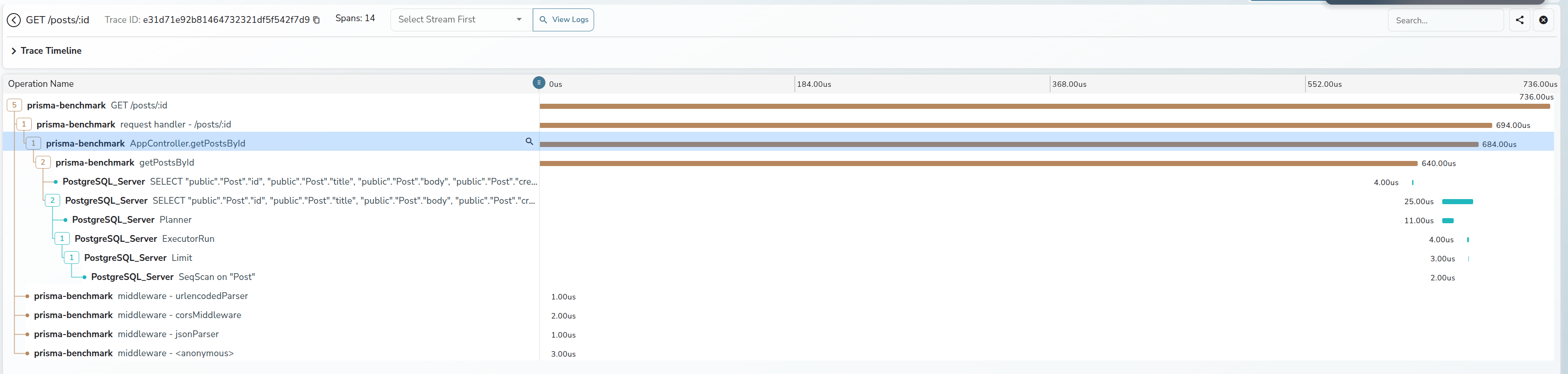
1 |
2026-02-22 07:56:38.681 GMT [190] LOG: execute s412381: SELECT "public"."Post"."id", "public"."Post"."title", "public"."Post"."body", "public"."Post"."createdAt", "public"."Post"."modifiedAt" FROM "public"."Post" WHERE ("public"."Post"."id" = $1 AND 1=1) LIMIT $2 OFFSET $3 /* method='GET',route='%2Fposts%2Fff4ccd6d-2c15-4979-a5f3-0c27e4e2f169',route_pattern='%2Fposts%2F:id',traceparent='00-e984180b391935fbdf2b1e1f6f3b2b12-1286ff6754fbbc57-01' */ |
通常来说,这样的语句已经能在我们常见的数据库调试流程中已经起到很大的帮助了,可以查到某一条慢 SQL 的来源,上下文等信息
但是这就够了吗?我们能不能把数据库也接入到 OpenTelemetry 的 tracing 体系中来呢?我们能不能在数据库的层面上看到整个调用链的 tracing 信息呢?
那没有问题的,这里以我现在更熟悉一点的 PostgreSQL 生态举个例子
Datadog 之前有一个工作,他们在 PostgreSQL 上实现了一个扩展叫作 pg_tracing https://github.com/DataDog/pg_tracing
通过使用 PostgreSQL 的一些扩展点
然后配合一些环形缓冲区和共享内存,就可以在数据库层面上实现一个 tracing 的功能了,这样我们就可以将 PostgreSQL 接入到 OTEL 生态中了。当然这个库的实现里面有不少小技巧,改天可以单独写个文章来聊聊
MySQL 虽然内部的实现是一坨,但是我想如果要在 MySQL 上实现类似的功能应该工作量也不会太大,
最终的效果如下所示
差不多就这样
大家都在写各种 AI/Agent 的文章的时候,我还在搞点这种 old school 的东西。恍惚间看到我的前方有一个巨大的风车。But anyway, 我喜欢这些东西, 这就够了
祝大家看的开心。
2026-01-01 23:00:00
每年都会选一句话作为年终总结的标题,去年是“本当の僕らをありがとう”,今年我选择“笑ってほしくて”。
这句话出自 《葬送的芙莉莲》的片尾曲《Anytime anywhere》。
愿你露出笑容
可能是我想对逝去之人,逝去的猫说的,可能也是他们想对我说的
也是我想对所有看到这篇文章的人说的
实际上一度想放弃写这篇文章,因为总是会害怕。今年在生死边缘搏战了许久。但终究是没有挽留住。每次想起点点滴滴时,总会不免破防
但是就如同歌词所说
こんなに胸が痛いのは/胸口传来的痛楚
あなたといた証かな/是与你同在的证明
那么所以还是要写点什么来纪念这特殊的2025, 也是 saka 的2025
今年生活中最大的事件就是猫咪的过世。小熊是我们在2023年从小区收养的猫咪。一最开始就给上了强度,重度口炎+肾衰。然后后续情况稳定后带回家进行日常的治疗。
而在24年经过一整年的折腾(开腹两次,病危三次),25年年初医生终于说可以两月复查后,我们以为小熊还能陪伴我们很长时间
但是事与愿违,在6月份过完到家纪念日后,小熊的状态就时好时坏。在8月份最后一次住进医院后,虽然期间还是有好转的时候,但是整体情况还是急转直下。最终我们选择放他离开
很难说,小熊的离去对我的打击是怎么样的。我同事说感觉我从中恢复过来还蛮快的。不过中个泪流时分也只有自己知道(其实写这篇文章的时候也是在默默流泪)
今年也是我好友离开我的第五个年头。恍惚间,我已经比他大了
君埋泉下泥销骨,我寄人间雪满头
不得不说古人是真的会写啊。
聊点开心的,今年我的日常生活比去年又丰富了很多。史无前例的,saka 获取了,他的,第一个全成就游戏!所以 2025 saka 严选最佳游戏的是?
是《空之轨迹 1st 重制版》
对不起 P5R,我也很爱你的(

今年也还在继续的拍照,买了 Z135 F1.8S 圆神,Z105 F2.8 百微,Z35 F1.2S 三个头,在摄影器材的路上越走越远,整体的快门数快 10w 了,整体以猫狗为主。某种意义上来说,我很庆幸用相机记录下了小熊这几年最精彩的时光
今年对于我来说另一个在最大的改变就是,我去了出来能去的最远的地方——日本
我精神图腾中的几大支柱(奥特曼,摇曳露营)都发源自日本,而我第一次出国便是去日本(某种意义上算冥冥之中的一种巧合)
在日本出差的这两周里,解锁了很多新奇的体验。去秋叶原爆米,去抚子的故乡爆米,在出租车上和司机一起唱奥特曼主题曲,和好友一起逛街爆米,和同事一起去热海合宿,见了好看的海边,去了沼津,吃了好吃的海鲜饭等等等。
某种意义上今年开启了我过去很多人生中未曾想过的体验。也让我坚定的了一个想法、
人与人的欢乐实际上是可以相通的

感情进入了第七个年头。如果要为今年的感情沉淀一个主题的话,那可能就是四个字,生死相依
小熊走前的一个月,我们在医院陪护。仪器的滴鸣声,时而奔走的医护。时而逝去的生命。那种氛围真的很压抑
这种时候,两个人的相互的守望,可能是枯燥且祈祷着奇迹发生的日子里,已然发生少数的奇迹。
小熊离去后,我们两也久违的带着小狗出远门去散心,去一起给小狗拍了很多好看的照片,一起救助了其余的小猫,一起给医院捐献了设备。
能在人群中遇到彼此守望的伴侣,本身已然是奇迹
今年年初在朋友邀请下,我加入了一家 AIGC 创业公司,负责一些 infra 上的工作。这算是我职业生涯一个全新的转折点。
如果说这里面最大的感受是什么,那就是我可能在之前聊过的,身份转变所带来的更多的责任与事情。
先聊聊务虚的部分,往常我只需要 focus 在具体的事情的落地,可能其余的东西都会有人帮我兜底。而我今年开始成为一个试图去帮助其余同事能够更好落地事情的人。说实话这种身份上的转变实际上会让你有很多想法转变。就如同我和团队成员 1:1 沟通时我一直在问的一个问题一样“你觉得我还能做什么,能帮助你落地现在的事情?”。很多时候我去思考事情的时候,我不能仅考虑这个事情本身,而是我需要去思考这个事情怎么样才能够帮助团队/同事实现更好的价值。
与此同时,我的职责以及角色会变得更多元化。这一点也是需要走出舒适区。比如今年我在公司做了很多涉及到 DBA 和搜索相关的工作。严格来说,这一部分工作其实离我的好球区实际上很远,但是如果一个事情是重要的,同时当下没有人比我更擅长这件事(换句话说让我做不会是最坏的结果),那么我就需要去承担起这份责任。
接着是务实的部分,如果要说今年很有成就感的事情的话,就是在加入公司后,从头开始做稳定性相关的建设,且收获颇丰。无论是在多次互联网 infra 大范围 crash 后我们能在最短的时间内恢复业务,还是给我们的业务带来了实际上的稳定性与性能提升。我所做的工作都能直接的作用在用户价值上。某种意义上来说,这也是人生的一件幸事
以上都是好的 part,坏的 part 也不是没有,那就是
教练,我想写代码
我现在写代码基本上只能靠工作之外写写代码来保持手感和练手,呜呜呜呜呜,我真的好想转岗去写代码啊(
不过这也不算坏事,我现在非常享受业余时间写代码的生活,所以今年在社区的贡献比去年多了不少,包括把自建图床项目的代码拾掇了很多,给 CPython 的 JIT 贡献了不少代码。也让自己名字第一次在官方文档里留下了痕迹。
如果说明年有什么想法的话,简单的说就是在工作上带好团队,能够继续突破我自己的舒适区。以及希望我能给 CPython 下一阶段的 JIT 贡献更多的代码(其实有一些想法,正好趁着元旦假期梳理一下)
啊,突然想起,我26年还得好好学学 GPU 相关的编程的东西,说实话学习新的东西真的是非常开心的一件事!
算是凑个热点,聊聊我对 AI 的看法。
很多人都会陷入一种焦虑,“AI 会不会替代我自己”
我自己的看法愈发的清晰,AI 时代会让人的价值更大,而不是被消泯
这里的逻辑很简单,AI 让一切都变得更为高效,内容的生产更为高效,开发效率更为高效,公司的形态更为灵活,在这种情况下,传统的很多东西在 AI 时代都面临的新的挑战。比如我举几个例子
对于愈发高效的内容生产效率,UGC 等形态的 AI Startup 会面临越来越大的 anti nsfw 的合规的挑战
而对于算力的愈发的渴求,边缘 GPU 算力的管控与接入也愈发成为一个重要的课题
AI 带来的生产力提升其实会让人的价值在这个时代更为凸显,而不是被消解
差不多就是这样吧。过去一年有过不少很多的泪水,也有过很多的难眠之夜,也有过很多的快乐。
坦白来说能挺过这一年,是因为身边有着很多的陪伴,有我女朋友,有一群好朋友,有一群好同事。
每一个人的陪伴加上生活中辛酸苦辣甜汇聚在一起就成为了2025年的 saka,或者是 saka 的2025。
曾经想对于以后试图列出很多的展望,但是死生经历过一轮后,觉得剩下的都不太重要了
如同标题一样,
笑ってほしくて/愿你露出笑容
愿我们每一个人都能以笑容度过2026年的每一天
一万年太长,我们只笑今朝(
新年快乐!
2025-10-03 04:00:00
最近刚把空轨 1st 打通关。差不多国庆假期也要结束了,要开始准备接下来的学习和工作了。趁着这个机会,写点东西,当个迟到的 PyCon China 2025 的总结吧
其实去年在结束去年的会议后,我就在考虑要不要彻底退出 PyCon China 一段时间。原因其实也很简单,太累了。不过我向来是个很拖延癌的人。恰逢那时候正在职业的变动期,所以想着要不要再看看。
今年来了一家 AIGC 公司做 infra,说实话我干的还蛮开心的。每天都会学习新的东西。状态相比于去年好了不少(除了每天都需要和该死的 Any 做斗争),所以一度准备继续参加今年的 PyCon China
不过到了筹备期后,原本的计划突生变故。陪伴需求的猫咪病危,去世。一直在医院通宵,陪护以及最终要面临的生死别离。对我的精神和体力造成了极大的消耗。是否继续参加今年的 PyCon China 也成为一个问题。
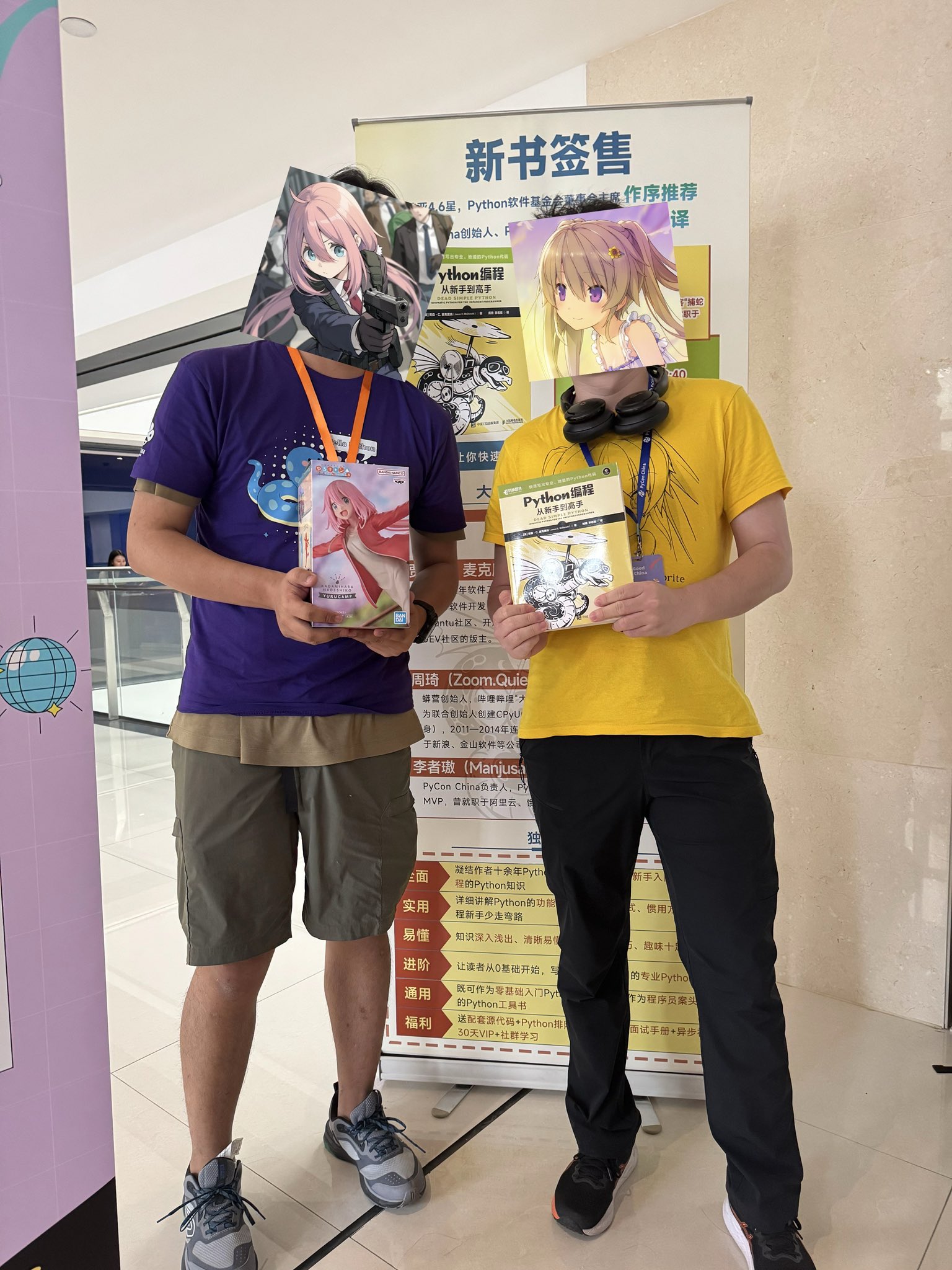
不过最终还是决定参加了。今年突然出版社那边给我加了一个活,我翻译的书要在现场签售。这就又成为我心里一个新的疑问:嘛,真的会有人来买吗?
嘛,其实这也是每年在参加 PyCon 时都会有的自我怀疑,我真的有资格在这里吗?我讲的东西真的会有人听吗?
不过做了最终的决定那么就继续做吧。所以今年还是给了一个白银赞助+一个主题演讲。
时间过得很快,转眼到了会议前一天,临上飞机前我还在被 AWS 的傻叉 OpenSearch 折磨。下飞机后 yihong,piglei,空想家,jay 他们去开 impact 了。好好好开 impact 不带我是吧。我就孤零零的跑去了酒店。有人演讲前12h文件夹都还没建是谁我不说。
在酒店顶了几个小时把 PPT 赶完,工作收个尾。勉强睡了2h,然后就去会场了。
今年比较轻松的是早上的主持不用我了,我只要负责暖场一下。不过临开场前发现 C 会场的 PPT 还没收,然后摇了晚枫帮忙。
暖场还是我每年的保留节目,Saka 三问.jpg:
看起来效果还不错。暖场完我就跑出去了。不过卧槽,今年怎么这么多人来单杀我,妈耶社恐狂哭了。
不过说实话,在经历生死一圈后,和老朋友打打闹闹,认识一下新朋友,还是蛮开心的。特别是很多人过来说我影响了他们,我是他们的偶像,他们从我的博客和分享里学到很多的时候。我一直以来的疑惑也得到了解决。虽然说人的自我认同最理想应该是内源性的,但是大家的认可也真的会让我很开心。
哦对了,还有很多人说他们也很喜欢摇曳露营!

值得一提的是,我司的宝藏同事从日本来一起面基了(是的,我们是 Remote 公司),还给我带了手办
当然有某屑 HR 说要来参会结果早上睡过了,是谁我不点名了
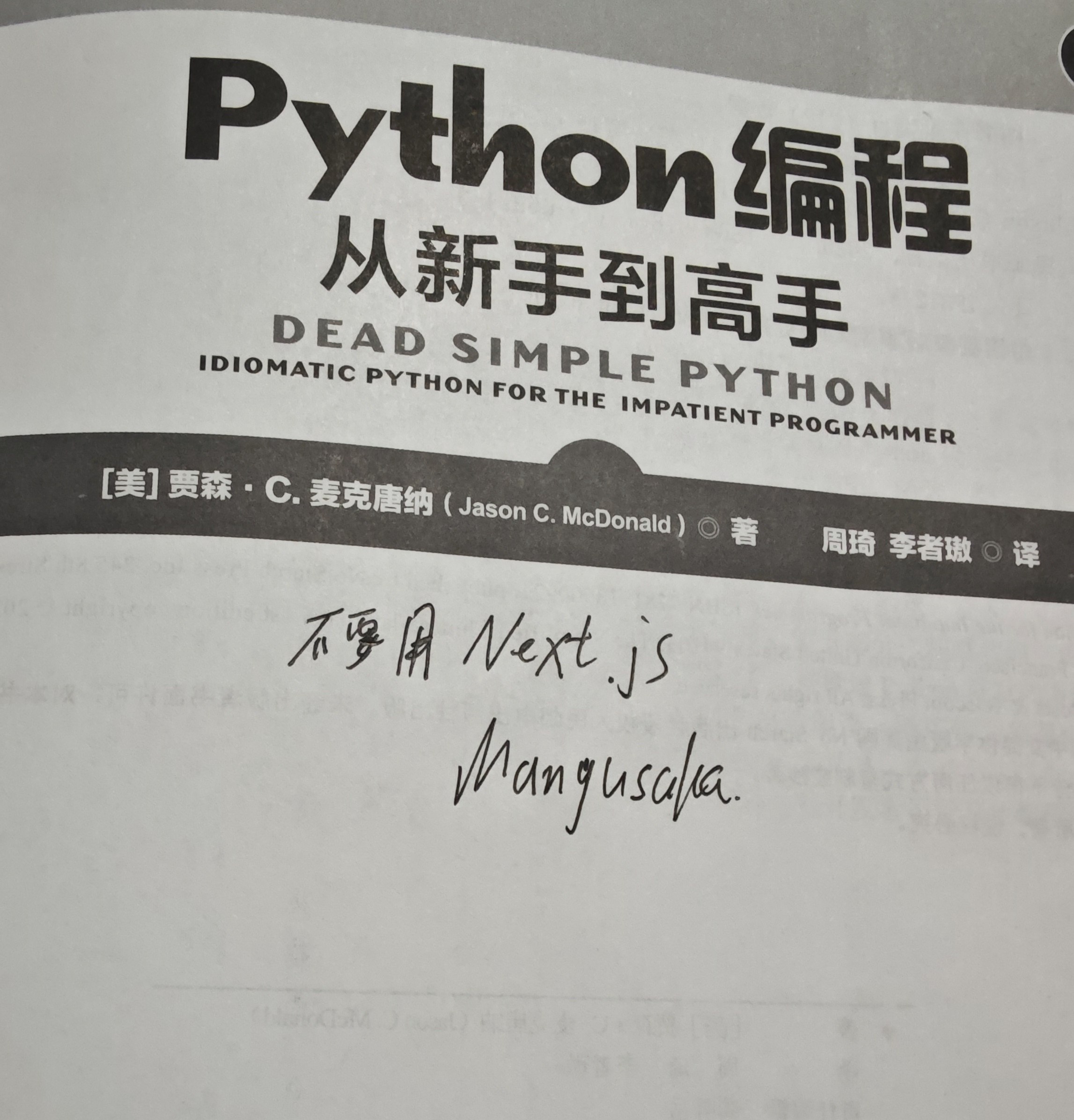
上午的时间其实过去的很快,很快就结束了。然后我就来到了签售地方。出乎意料的,有很多人都来了,有来捧场的老朋友们,有刚刚线下刚对上号的新朋友们。大家一起打打闹闹,我用我的丑字写了很多祝福,也有很多杂话。要说哪一句最真心,那我觉得是“不要用 Next.js”罢。
签售完火急火燎的吃完盒饭,抽烟的时候遇到师父,我开始基情的抚摸他的胸肌,这可能算是每次我们师徒相聚的仪式感了。问他了一个问题:你现在还需要我帮你收尸么?这个出处源自于我们之前约好他要是自杀我会来帮他处理后事。他想了想说,我们不如想想怎么活到150岁吧。很好,很强大,我很喜欢的回答。那我就当不会了。
后面纯爷也来加入了聊天,我顺便向他倾诉了一下把 PostgreSQL 当 MongoDB 用的痛苦。纯爷也只能用爱莫能助的眼光看看我
下午 C 会场实际上因为我需要抽烟提神迟到了几分钟,yihong 帮我暖场缓解尴尬,不得不给他磕一个,以及 yihong 抱起来手感很好,建议网友有条件的可以去试试
下午到我的时候其实因为控场的原因给我的时间比预期的要短一些,所以我临时调整了一些内容。要上去讲的时候,发现很多人都从其余会场赶了过来,算是非常满足了。在 QA 的时候,我给大家说我现在在一家用着 Node.js 写着 Any,把 PostgreSQL 当 MongoDB 用,以及还用着 GraphQL 的公司工作。大家一片会心一笑。我想我们屑 HR 大概今天在现场招不到人了罢
下午的时候,屑 HR 和我们在上海的另外一位同事也来,带来了我需要昏睡红茶零度可乐。说实话在一个 Remote 公司大家面基的机会还是很少的。理所当然,我成为公司群内表情包的一部分。该考虑下找屑 HR 要肖像费了
晚上散场后,去和沪爷阿蔡以及几个同事一起组了一个局。不过说实话拉着明天要去霓虹的两位同事去吃日式拉面算不算另一种职场 80?笑死
说实话今年 PyCon 的当天是我这两个月最快乐的一点,也许在很多年后我记不得了今年讲了什么,但是还会记得当天最简单快乐。
嘛,从18年到现在,7年过去了,我也从一个刚出校园的年轻人变成了一个老登。似乎很多东西都在变,但是很多东西又没变。
我还是很菜,但是我好像比之前影响了更多的人,帮到了更多的人?我还有很多东西不会,但是我好像能学的东西也更多了?还是会经历很多痛苦,很多迷茫,很多挣扎。但是生活似乎也还是一如既往的有着无限的希望与美好?
回北京后,一次吃饭时,我给我女朋友说,你知道吗?很多人说我是他们的偶像。我女朋友说:不,你是他们的榜样
是的,成为榜样,但是不要成为偶像。
这篇文章差不多写到这里。要到中秋了,除了祝大家中秋快乐,阖家欢乐以外。也祝大家每个人都能在这个快速迭代的世道里永葆初心。用 Piglei 老师的话说就是“老而不登”
这个世界唯有爱,希望,奥特曼与摇曳露营不可辜负,抚门!