2026-07-28 07:08:59
The latest issue of Paged Out! has an article by Stephen Hewitt “An off-line backup of your cryptographic key using playing cards.” The idea is to use a deck of 52 to store a 128-bit cryptographic key. To erase the key, shuffle the deck. Hewitt gives his algorithm for embedding a key, one that can be carried out manually but isn’t maximally efficient.
You could store a 225-bit key as a permutation of 52 cards because
log2(52!) = 225.581.
But then how would you number permutations so you could go from a number to a particular permutation and later decode the permutation to a number? Is this even practical? For a small number n, you could encode a number k < n by enumerating the first k permutations of a set of n items, and you could decode by enumerating permutations until you find the one you have. But this is completely impractical for large n, such as n = 52.
The process of mapping permutation to an integer is called ranking, and the mapping from an integer to a permutation is called unranking. How efficiently can rankings and unrankings be calculated?
Let n be the number of symbols being permuted. Then there are simple algorithms for ranking and unranking with respect to lexicographical order that have complexity O(n²) and more sophisticated algorithms that have complexity O(n log n). There are also O(n) algorithms that do not preserve lexicographical order.
The Permutations class in SymPy has methods unrank_lex and rank to unrank and rank permutations according to lexicographical order.
The notation the Permutations class uses requires a little explanation. For example, suppose we unrank 2026.
>>> from sympy.combinatorics import Permutation
>>> Permutation.unrank_lex(52, 2026)
Permutation(45, 47, 51, 48, 46, 50)
The output is not a full list of 52 numbers in permuted order; it is only a cycle. The notation refers to the permutation that sends 45 to 47, 47 to 51, …, 50 to 45 and leaves everything else fixed.
If we rank the permutation given above, we get 2026 back.
>>> Permutation.rank(Permutation(45, 47, 51, 48, 46, 50))
2026
Note that we didn’t say how many elements (45, 47, 51, 48, 46, 50) is a permutation of. Because of lexicographical order, the rank would be the same whether we viewed this as a permutation of 52 objects or of more objects.
Now let’s do something larger. Let’s generate a 220-bit number and encode it as a permutation.
>>> n = random.getrandbits(225)
>>> a = Permutation.unrank_lex(52, n)
>>> n
40234719030664563684489051530416964877785781669439875437823431388841
>>> a
Permutation(0, 25, 32, 15, 8, 28)(1, 48, 34, 14, 10, 51, 38, 31, 21, 5, 42, 47, 29, 26, 46, 30, 50, 49, 37, 22, 18, 23)(2, 45, 17, 20, 36, 40, 11, 4, 7, 41, 33, 3, 43, 44, 19, 16, 35, 39, 12, 6, 9)
>>> Permutation.rank(a) == n
True
Now just for fun, let’s display the permutation above applied to a standard (French) deck of 52 cards. As explained here, symbols associated with these cards have a range of Unicode values. By printing these values, we can visualize the permuted deck.
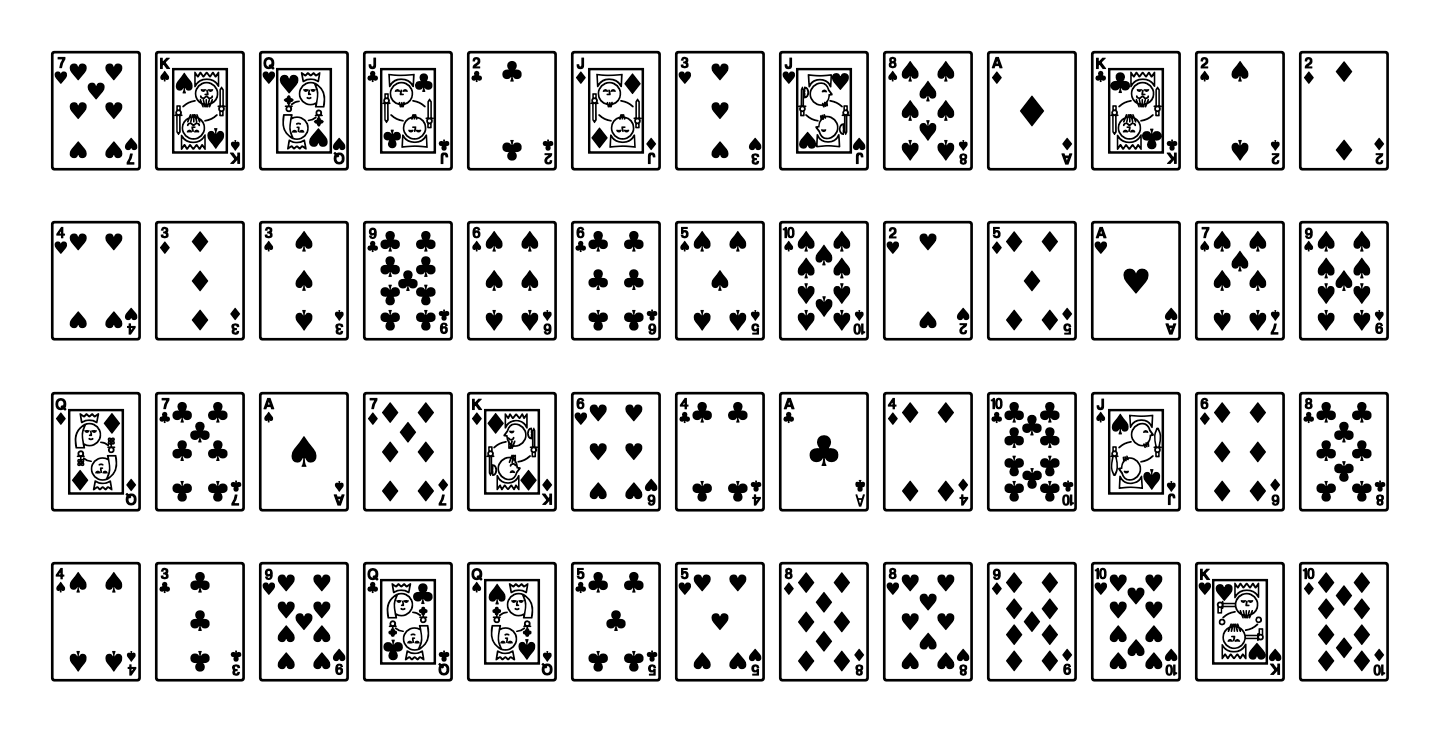
Here’s the code that made the image above.
spades = list(range(0x1F0A1, 0x1F0AF))
spades.remove(0x1F0AC) # take out the knight
cards = [s + 16*i for s in spades for i in range(4)]

a = Permutation.unrank_lex(52, n)
p = a(cards)

for i in range(4):
    for j in range(13):
        print(chr(p[13*i + j]), end="")
    print()
The code above is plenty fast, but Permutation has methods rank_nonlex and unrank_nonlex that run in O(n) time, which could be useful for n much larger than 52.
2026-07-28 00:03:44
My post from yesterday on permutation roots ends with a Mathematica code for finding the probability that a permutation of n elements has a kth root. This is done by finding the coefficient of xn in the generating function

I wanted to say more about this, and look at implementing the same code in SymPy. I was curious how well SymPy would do because I’ve noticed that LLMs often generate SymPy code since it’s an open source CAS.
Wilf [1] describes the infinite product above as the exponential generating function (egf) of f(n, k), the number of permutations of n objects that have a kth root. Since egfs have a n! term in the denominator, this is also the ordinary generating function (ogf) of the probability that a randomly chosen permutation on n objects has a kth root.
My first attempt at using Mathematica to probe the generating function was
expq[x_, q_] := MittagLefflerE[q, x^q]
p[n_, k_] :=  SeriesCoefficient[
    Product[expq[x^m/m, GCD[m, k]], {m, 1, Infinity}], {x, 0, n}]
This hung forever when I tried to use it on a small example. I realized, but apparently Mathematica did not, that Infinity could be replaced by n since terms higher than n do not contribute to the coefficient of xn. With that change, the code ran quickly.
This morning I tried converting the Mathematica code to Sympy; Claude did this in one shot. I also reproduced the table of f(n, k) values on page 150 of [1] to test the code. Since Wilf tabulated f(n, k), not f(n, k)/n!, I multiplied the results by n!.
Here is the output:
k = 2 [1, 1, 3, 12, 60, 270, 1890, 14280, 128520, 1096200]
k = 3 [1, 2, 4, 16, 80, 400, 2800, 22400, 181440, 1814400]
k = 4 [1, 1, 3, 12, 60, 270, 1890, 13020, 117180, 1039500]
k = 5 [1, 2, 6, 24, 96, 576, 4032, 32256, 290304, 2612736]
k = 6 [1, 1, 1, 4, 40, 190, 1330, 8680, 52920, 340200]
k = 7 [1, 2, 6, 24, 120, 720, 4320, 34560, 311040, 3110400]
and here is the SymPy code. I edited the main but the rest is verbatim from Claude.
from sympy import symbols, gcd, factorial, Rational, S

x = symbols('x')

def expq_coeffs(m, q, n):
    """
    Truncated (degree <= n) series coefficients of
        expq(x**m/m, q) = MittagLefflerE(q, (x**m/m)**q)
    Since q is a positive integer:
        E_q(y^q) = sum_j y^(q*j) / (q*j)!
    with y = x**m/m, so the term of degree m*q*j has coefficient
        1 / ( m**(q*j) * (q*j)! ).
    Returns a list c[0..n] of coefficients.
    """
    c = [S.Zero] * (n + 1)
    j = 0
    while m * q * j <= n:
        deg = m * q * j
        c[deg] += Rational(1, m**(q * j) * factorial(q * j))
        j += 1
    return c

def poly_mult_trunc(a, b, n):
    """Multiply two series (lists of coeffs, index = degree) truncated to degree n."""
    c = [S.Zero] * (n + 1)
    for i, ai in enumerate(a):
        if ai == 0:
            continue
        max_j = n - i
        for j2 in range(max_j + 1):
            bj = b[j2]
            if bj != 0:
                c[i + j2] += ai * bj
    return c

def p(n, k):
    """
    SymPy equivalent of:
        expq[x_, q_] := MittagLefflerE[q, x^q]
        p[n_, k_] := SeriesCoefficient[
            Product[expq[x^m/m, GCD[m, k]], {m, 1, n}], {x, 0, n}]
    """
    result = [S.Zero] * (n + 1)
    result[0] = S.One
    for m in range(1, n + 1):
        q = gcd(m, k)
        factor = expq_coeffs(m, q, n)
        result = poly_mult_trunc(result, factor, n)
    return result[n]

# example
if __name__ == "__main__":
    for k in range(2, 8):
        print("k =", k, [factorial(n)*p(n, k) for n in range(1,11)])
[1] Herbert Wilf. Generatingfunctionology. Available online here.
The post Counting permutations with roots first appeared on John D. Cook.2026-07-27 23:34:05
It’s well known that you can convert the base 16 (hex) representation of an integer to the base 2 (binary) representation by simply converting each digit from hex to binary. For example,
CAFEhex = 1100 1010 1111 1110two
I imagine it’s less well known that you can do the same thing with floating point numbers.
I wanted to find the binary representation of a floating point number using Python, and discovered that it has no function to do this. However, there is a method on floats to show a hex representation. For example, here’s the hex representation of π.
>>> import math
>>> (math.pi).hex()
'0x1.921fb54442d18p+1'
Curiously, the p+k part at the end is an exponent of 2, not an exponent of 16. So after we convert 1.921fb54442d18 to binary, we’ll need to multiply by 2, i.e. move the fractional point one space to the right.
So first we convert 1.921fb54442d18hex to binary by converting 1, 9, 2, etc. each to binary.
1.1001 0010 0001 1111 1011 0101 0100 0100 0100 0010 1101 0001 1000two
Then after shifting the fraction point to account for the p+1 part we have
π = 11.001001000011111101101010100010001000010110100011000two
You could use Python’s bin() function to convert the fractional part, interpreted as an integer, to hex, though you may need to pad with 0 bits. For example,
>>> (1.03).hex()
'0x1.07ae147ae147bp+0

>>> bin(0x7ae147ae147)
'0b1111010111000010100011110101110000101000111'
The binary representation of 1.03ten is
1.000001111010111000010100011110101110000101000111two
We added a total of five zero bits, four for the 0 after the fractional point and one for converting 7 to 0111two.
The post Printing floating point numbers in binary first appeared on John D. Cook.2026-07-27 04:32:02
Let σ be a permutation on n elements. If there is a permutation τ such that applying τ twice has the same effect on the list of elements as applying σ once, we say σ = τ² and τ is a square root of σ.
If we let our n elements be the integers 0 through n − 1, then we can represent permutations by what they do to this list of numbers. In Python as a tuple of length n and compose permutations with the following function:
import itertools

def compose(sigma, tau):
    "Return the composition σ ∘ τ (apply τ first, then σ)."
    return tuple(sigma[j] for j in tau)
We can always construct permutations that have square roots by squaring a permutation. If we run the following code
tau = (3, 1, 4, 5, 2, 0)
sigma = compose(tau, tau)
we find σ = (5, 1, 2, 0, 4, 3), and by construction (3, 1, 4, 5, 2, 0) is a square root of &sigma, though it’s not the only one.
The following code shows that σ has four roots.
import itertools

def numroots(sigma):
    n = len(sigma)
    c = 0
    for tau in itertools.permutations(range(n)):
        if sigma == compose(tau, tau):
            c += 1
    return c

print( numroots(sigma) )
print( numroots( (1, 2, 3, 4, 5, 0) ) )
It also shows that the rotation (1, 2, 3, 4, 5. 0) has no roots.
The function numroots has runtime proportional to n! and so it’s not practical for large permutations. There is a theorem that says a permutation σ has a square root if and only if the number of cycles it has of every even length is even. See [1].
We can also define cubes and cube roots of permutations, and higher powers and roots.
How common is it for permutations to have square roots, or cube roots, etc.? If you pick a random permutation on n elements, what is the probability that it has a kth root?
This is a hard question in general, but it is equivalent to finding the coefficient of xk in the infinite product
This is theorem 4.8.3 in [1]. This theorem was the motivation for writing about expq in the previous post.
Although the product is infinite, there’s no need to compute terms in the product that only contribute powers of x higher than you’re interested in. The following Mathematica code will compute the probability that a permutation on n elements has a kth root.
expq[x_, q_] := MittagLefflerE[q, x^q]
p[n_, k_] :=  SeriesCoefficient[
    Product[expq[x^m/m, GCD[m, k]], {m, 1, n}], {x, 0, n}]
So, for example, the probability that a permutation of 10 elements has a square root is 29/96.
[1] Herbert Wilf. Generatingfunctionology. Available online here.
The post Permutation roots first appeared on John D. Cook.2026-07-27 02:20:36
The function expq(x) is defined by taking the power series for exp(x) and keeping only the terms whose index is a multiple of q. For example, exp2(x) keeps only the even-numbered terms in the exponential power series and so equals cosh(x).
![]()
In general,
![\exp_q(x) = \sum_{n=0}^\infty [q \mid n] \frac{x^n}{n!} = \sum_{n=0}^\infty \frac{x^{nq}}{(nq)!}](https://www.johndcook.com/expq2.svg)
The first sum uses Iverson’s bracket notation: a Boolean expression in brackets denotes the function that returns 1 when the expression is true and zero when it is false. Here the bracket equals 1 when q divides n and is zero otherwise.
Let ω = exp(2πi / q). Then

This lets us find closed-form expressions for expq(x). For example, when q = 4, ω = i and
![]()
Here’s a proof of the identity above:
![\begin{align*} \frac{1}{q} \sum_{k=0}^{q-1} \exp(\omega^k x) &= \frac{1}{q} \sum_{k=0}^{q-1} \sum_{n=0}^\infty \frac{\omega^{kn}x^n}{n!} \\ &= \sum_{n=0}^\infty \left( \frac{1}{q} \sum_{k=0}^{q-1} \omega^{kn}\right) \frac{x^n}{n!} \\ &= \sum_{n=0}^\infty [q \mid n] \frac{x^n}{n!} \\ &= \exp_q(x) \end{align*}](https://www.johndcook.com/expq5.svg)
In the proof we used the identity
![\frac{1}{q} \sum_{k=0}^{q-1} \omega^{kn} = [q \mid n]](https://www.johndcook.com/expq6.svg)
which is important in deriving the properties of the discrete Fourier transform.
The first time I saw the function expq(x) was in differential equations, though I didn’t know at the time the function had a name.
When a course in differential equations gets to power series solutions, a common example or homework problem is to solve
![]()
for k = 3 or 4, i.e. to find a function that equals its third or fourth derivative.
If the initial conditions are
![]()
and
![]()
the unique solution to
![]()
is y(x) = expk(x).
Mathematica does not have a built-in function implementing expq(x), but it does have an implementation of the Mittag-Leffler function, and so thanks to a relation between this function and expq(x) you can implement the latter as
expq[x_, q_] := MittagLefflerE[q, x^q]
The first time I saw the notation expq(x) was in combinatorics. I had intended to include an application from that book here, but I make that the topic for the next post.
The post exp_q first appeared on John D. Cook.2026-07-25 21:37:30
I was working with a wide spreadsheet from a client the other day and I had to convert between Excel column labels and column numbers. I had never paid attention to how Excel labels columns and implicitly thought it was base 26 using letters rather than digits. But then I realized that’s not right.
Excel labels columns A through Z, then AA through AZ, then BA through BZ, etc. If this is base 26, then does A correspond to 0? That could work for A through Z, but then what about AA? Then you’d have to say the first A corresponds to 26 but the second A corresponds to 0.
Does Z correspond to 0? If so then the column numbers would be 1 through 25, followed by 0, then 27. And it would mean that columns ZA through ZZ are the same as A through Z.
In fact nothing in Excel column labeling corresponds to 0. The labels cannot be interpreted as a positional number system.
There’s a name for this kind of number system: bijective base 26. The concept extends generally to bijective base b for any positive integer b. The idea is ancient, but the name was coined recently. It has also been called k-adic numbering. For most of history it didn’t have a name.
The motivation behind the name bijective base b is that there is a bijection (a one-to-one correspondence) between these symbols and positive integers; there’s no possibility of leading zeros that would keep the mapping from being a bijection, unlike say 7 and 07 representing the same number.
Before 2007, an Excel file could have a maximum of 28 = 256 columns, and so the largest column label was IV.
Then in 2007 the column limit was increased to 214 = 16,384 and the largest column label is XFD.
Converting from column labels to integers is easy; going the other way is a little more complicated.
letter_to_ordinal = lambda c: ord(c) - ord('A') + 1
ordinal_to_letter = lambda n: chr(ord('A') + n - 1)

def label_to_num(label):
    label = label.upper()
    n = 0
    for c in label:
        n = n*26 + letter_to_ordinal(c)
    return n

def num_to_label(n):
    letters = []
    while n > 0:
        n, remainder = divmod(n - 1, 26)
        letters.append(ordinal_to_letter(remainder + 1))
    return ''.join(reversed(letters))
Here’s an online calculator based on the code above.
The following code verifies the assertions above about the maximum number of Excel columns over time.
assert(num_to_label(256) == "IV")
assert(label_to_num("IV") == 256)

assert(num_to_label(2**14) == "XFD")
assert(label_to_num("XFD") == 2**14)
The conversion routines are not limited to actual Excel labels but work for arbitrarily large integers and bijective base 26 representations. For example, the following code shows that the bijective base 26 representation of Avogadro’s number is MUAEKAUDYDXEWOSDD.
avogadro = 602_214_076_000_000_000_000_000
assert(label_to_num(num_to_label(avogadro)) == avogadro)
print(num_to_label(avogadro))