2026-05-29 23:00:42
Welcome to HackerNoon’s Projects of the Week, where we spotlight standout projects from the Proof of Usefulness Hackathon, HackerNoon’s competition designed to measure what actually matters: real utility over hype. \n \n Each week, we’ll highlight projects that demonstrate clear usefulness, technical execution, and real-world impact - backed by data, not buzzwords.
This week, we’re excited to share three projects that have proven their utility by solving concrete problems for real users: Yaeum, XColdPro, and EquipmentStack.
\
:::tip Want to see your own project spotlighted here?
Join the Proof of Usefulness Hackathon to get on our radar.
:::
Yaeum is an innovative language learning app that allows fans of K-pop and K-drama to learn Korean directly from their favorite content using generative AI and machine learning.
Search for a Korean song, drama, or movie, and Yaeum will provide an in-depth analysis of the text, sentence by sentence, and set up a personalized vocabulary list to make memorizing new words easy. To achieve this, Yaeum taps into several open sources third party apis and uses generative AI and machine learning to analyze the texts and provide grammatical explanations as well as vocabulary.
Proof of Usefulness score: +74 / 1000
\

\
:::tip See Yaeum’s full Proof of Usefulness report
Read their story on HackerNoon
:::
XColdPro is a patent-pending, hardware-agnostic cold storage software designed to protect both cryptocurrency keys and the host machine holding them, solving critical issues around digital asset inheritance and OS-level threat defense.
XColdPro leverages Python and Electron to deliver a cross-platform experience, secured by robust AES-256-GCM encryption and PBKDF2 with 500K iterations. The tech stack is uniquely built to operate in a fully air-gapped, no-cloud environment, while utilizing scheduled task watchdog architecture and OS-level behavioral monitoring to seamlessly integrate threat intelligence.
Proof of Usefulness score: +52 / 1000
\

\
:::tip See XColdPro’s full Proof of Usefulness report
Read their story on HackerNoon
:::
EquipmentStack is a newly launched, niche content platform focused on detailed athlete equipment specifications. The platform helps enthusiasts find exactly what the pros use, diving into the labor-intensive data gathering that earned them their recent Proof of Usefulness score.
To build and manage its extensive content repository, EquipmentStack utilized WordPress as its foundational technology. Choosing WordPress allowed it to rapidly deploy a custom, SEO-friendly site that is perfectly suited for managing a highly structured database of gear and athletes without unnecessary technical overhead.
While the project is in its infancy with no verifiable user traction yet, the live site demonstrates high-quality, labor-intensive data gathering that offers genuine utility to enthusiasts.
Proof of Usefulness score: +35 / 1000

\
:::tip See EquipmentStack’s full Proof of Usefulness report
Read their story on HackerNoon
:::
It's our answer to a web drowning in vaporware and empty promises. We evaluate projects based on: \n ▪️ Real user adoption \n ▪️ Sustainable revenue \n ▪️ Technical stability \n ▪️ Genuine utility
Test your project’s usefulness and submit your report on Hackernoon before August 10, 2026, to compete for over $150,000 in cash prizes and software credits.
Projects score from -100 to +1000. Top scorers compete for $20K in cash and $130K+ in software credits.
You’ll be in good company. The hackathon is backed by teams who ship production software for a living - Bright Data, Neo4j, Storyblok, Algolia, and HackerNoon.
\

\
1. Get your free Proof of Usefulness score instantly \n 2. Your submission becomes a HackerNoon article (published within days) \n 3. Compete for monthly prizes \n 4. All participants get rewards
Complete guide on how to submit here.
:::tip 👉 Submit Your Project Now!
:::
\ That’s all for now.
Until next time, Hackers!
2026-05-29 22:59:59
AI is not a great equalizer. It is a great amplifier. It amplifies what you already are — for better and for worse.
2026-05-29 22:29:59
Now remember how PCA collapses data with 100 dimensions into a single dimension, wouldn't it be cool if this dimension was interpretable. For example, let's say the 100 columns were like stress, smoking frequency, alcohol ml etc etc.. you see where I am going with this, the final dimension would be something like cardiac arrest or premature demise. On that cheery note, let's figure out how PCA can actually be used to label this reduced dimension.
2026-05-29 22:16:00
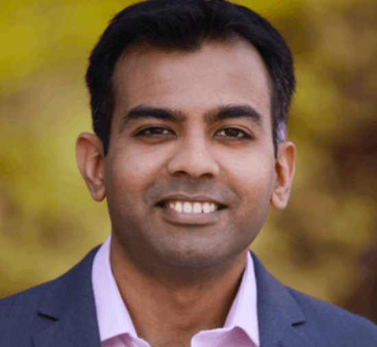
For most people, the US immigration system feels like a black box. You submit documents, you wait and you hope. The rules shift without warning. The timelines stretch. The costs climb. And if something goes wrong, figuring out why can take months and thousands of dollars in legal fees.
Swatilina Barik decided that did not have to be the case.
A seasoned practitioner with 10+ years of hands-on experience inside immigration strategy, Barik has spent considerable time watching the same problems repeat themselves. Applicants arriving underprepared. Petitions filed with gaps that could have been caught early. Strategies chosen not because they were the best fit but because they were the most familiar. She did not see a system that needed a few upgrades. She saw one that needed to be rethought entirely.
That rethinking led to Visa Architect.
US immigration is not a single pathway. It is a sprawling web of visa categories, eligibility criteria, processing timelines and adjudication patterns that shift depending on country of origin, employer size, job role and a dozen other variables. Navigating it well has always required deep expertise and deep expertise has always been expensive.
Visa Architect changes that equation. The platform uses artificial intelligence to do what the best immigration strategists do but at a scale and speed that was not previously possible. It analyzes an applicant's profile, maps it against relevant visa categories, identifies potential weaknesses in a petition before it is filed and models how different approaches might play out given current adjudication trends.
The result is not just faster processing. It is smarter decision-making from the very beginning of the immigration journey.
There is no shortage of technology companies trying to automate legal processes. What makes Barik's approach different is where she started. She did not come to immigration as an outsider looking to apply a general-purpose AI tool to a new market. She came as someone who had already spent years inside the system, learning what actually trips applications up and what actually gets them approved.
That practical knowledge is embedded in Visa Architect in ways that a purely data-driven approach would miss. The platform understands not just the rules but the context around the rules. It reflects the kind of judgment that experienced practitioners develop over years and makes it accessible to a much wider range of users.
The impact of Visa Architect reaches across the immigration ecosystem.
For individual applicants, it means entering the process with a clearer picture of where they stand. They can understand which visa pathway is genuinely the strongest fit for their circumstances rather than defaulting to whatever their employer used for the last hire. They can see potential red flags in their documentation before a case officer does. They can make informed choices rather than hoping for the best.
For businesses, particularly smaller companies that lack dedicated immigration teams, it means access to a level of strategic analysis that was previously out of reach. A startup sponsoring its first international employee no longer has to navigate the process blind.
For immigration attorneys, Visa Architect is not a replacement. It is a resource. It handles the research-heavy analytical work that consumes hours of preparation time, freeing practitioners to focus on the judgment calls, the nuanced arguments and the client relationships where human expertise is irreplaceable.
What Barik is building points to something larger than a single platform. It reflects a fundamental shift in how AI can and should be applied to high-stakes professional fields.
For years the dominant approach was to automate simple tasks and leave complex ones to humans. What Visa Architect demonstrates is that AI built on deep domain knowledge can take on genuinely complex work, not by replacing human judgment but by expanding who has access to informed guidance in the first place.
The US immigration system is not going to get simpler. Policy changes, backlogs and evolving adjudication standards are a permanent feature of the landscape. But the tools people use to navigate that landscape are changing. Swatilina Barik is building some of the most important ones. \n
:::tip This story was distributed as a release by Sanya Kapoor under HackerNoon’s Business Blogging Program.
:::
\
2026-05-29 22:00:59
How are you, hacker?
🪐Want to know what's trending right now?:
The Techbeat by HackerNoon has got you covered with fresh content from our trending stories of the day! Set email preference here.
## What is Predictive Software Quality? Software Operations in the AI Era  By @playerzero [ 8 Min read ]
PlayerZero explains how predictive software quality helps enterprises prevent defects, reduce firefighting, and scale reliable software development with AI. Read More.
By @playerzero [ 8 Min read ]
PlayerZero explains how predictive software quality helps enterprises prevent defects, reduce firefighting, and scale reliable software development with AI. Read More.

By @scylladb [ 4 Min read ] New research reveals why companies ignore database risks until costs, latency, or outages force migrations—and what warning signs to watch. Read More.

By @tsivarev [ 7 Min read ] Where AI helps in ecosystem design, where it fails, and why human judgment must stay in the loop for trust, grants, reputation, and governance. Read More.

By @modulate [ 10 Min read ] Deepfake vishing surged 1600% in 2025. Most detection tools analyze text, not audio — and miss what matters. Here's how voice-native detection actually works. Read More.

By @webintelligencehub [ 7 Min read ] IP pool size is a marketing number. Learn which metrics matter when evaluating proxy providers, and what to look for on their websites before you spend a dollar Read More.

By @zbruceli [ 21 Min read ] Inside the biological tricks that let three-pound brains outlearn trillion-parameter machines — and the radical new architectures trying to close the gap Read More.

By @akashi-ghost [ 11 Min read ] AI is not alien or fake intelligence. It is accumulated human thought, culture, code, bias, and memory reflected back through machines. Read More.

By @macpaw [ 5 Min read ] MacPaw Research explains why macOS is severely underrepresented in public AI datasets and introduces GUIrilla, a framework for scalable Mac UI exploration. Read More.

By @arthurlazdin [ 6 Min read ] UB isn't a dark corner of C. It's what happens when a program steps outside its computational model — and the compiler, a perfect executor, follows the math. Read More.

By @syedahmershah [ 8 Min read ] I put Nous Research's hot new Hermes Agent framework through 5 brutal, multi-step tasks to see if it actually self-improves or just fails silently. Read More.

By @kumar96 [ 7 Min read ] Creating third-party integration is not a problem in OutSystems. It talks about web services, OAuth, and other security in APIs Read More.

By @joseh [ 4 Min read ] Kenshi and Kintaro are just a few of the characters that should be in Mortal Kombat 3. Read More.

By @mattleads [ 15 Min read ] A practical, working demonstration of 7 advanced Doctrine ORM strategies to eliminate the N+1 query problem in Symfony applications. Read More.

By @bennydoda [ 5 Min read ] AI agents will move so fast in establishing decentralised ecosystems for trading that regulators won't know where to start Read More.

By @notllmhallucination [ 12 Min read ] A review of context and memory issues in LLMs against the methods of AI startups to solve these in biological or biology-mimicking ways. Read More.

By @efimovov_5guqm5 [ 7 Min read ] MCP servers connect Claude Code to external tools. Use scopes correctly, keep credentials in env vars, and run mcp-scan on every new server. Read More.

By @huckler [ 7 Min read ] My system monitor with its own 9-layer AI between €3.8/h retail shifts. 55 GitHub stars, 260 downloads, 10 months solo. Here's everything it does. PC Workman. Read More.

By @qatech [ 7 Min read ] Learn how AI-generated code is shifting software QA toward continuous verification, agentic testing, and context-aware product quality systems. Read More.

By @vladlensk1y [ 4 Min read ] How I use AGENTS.md and a GitHub Action to catch low-effort AI-generated PRs before wasting maintainer review time. Read More.

By @apilayer [ 4 Min read ]
Discover 7 of the best SERP APIs for SEO and market research in 2026. Read More.
🧑💻 What happened in your world this week? It's been said that writing can help consolidate technical knowledge, establish credibility, and contribute to emerging community standards. Feeling stuck? We got you covered ⬇️⬇️⬇️
ANSWER THESE GREATEST INTERVIEW QUESTIONS OF ALL TIME
We hope you enjoy this worth of free reading material. Feel free to forward this email to a nerdy friend who'll love you for it.
See you on Planet Internet! With love,
The HackerNoon Team ✌️
.gif)
2026-05-29 22:00:46
Where founders share what they learn on the go. Read founder-related content: everything from challenges, success stories, leadership tips, to experiments.
 In this interview we speak with Alex Busarov the co-founder of Taelpay about Taelpay ecosystem a blockchain application developed by the team while operating in China. Tael consists of over
50,000 users in 500 cities, hundreds of products protected with NFC chips and
blockchain, all in cooperation with a long list of participating companies like Rakuten,
Nestlé, New Zealand Cherry Corp,and many more. The Tael ecosystem is anchored by
the Tael token which acts as a reward, loyalty, and marketing incentive for
participants in the ecosystem. Now lets delve straight into the interview!
In this interview we speak with Alex Busarov the co-founder of Taelpay about Taelpay ecosystem a blockchain application developed by the team while operating in China. Tael consists of over
50,000 users in 500 cities, hundreds of products protected with NFC chips and
blockchain, all in cooperation with a long list of participating companies like Rakuten,
Nestlé, New Zealand Cherry Corp,and many more. The Tael ecosystem is anchored by
the Tael token which acts as a reward, loyalty, and marketing incentive for
participants in the ecosystem. Now lets delve straight into the interview!
 Why Even Track Your Habits?
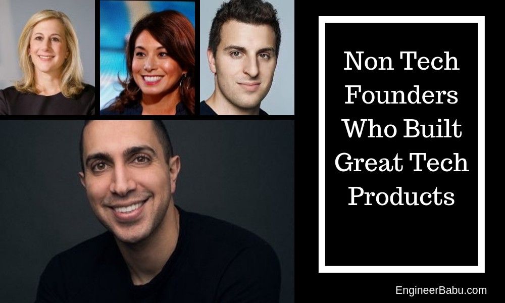 It might be surprising to some, but even non-technical startup founders have been behind great tech products like Tinder and AirBnB without the usual background
 A successful pitch starts with a well-thought-out pitch deck. And the "Why now" section is arguably one of the most important aspects of that deck.
 An exit strategy is often developed at an early stage and outlined in a business plan so that investors understand how they will receive a return of investments
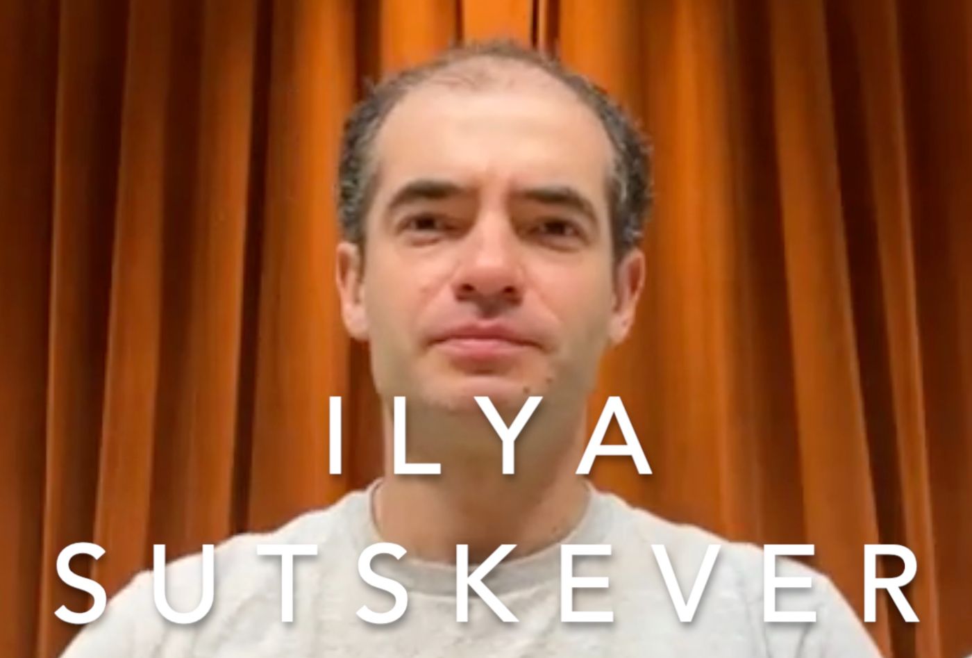 OpenAI cofounder and chief scientist Ilya Stuskever talks about ChatGPT and the promise of models like GPT-4
 Entrepreneurship definitely is one of the most misconceived terminologies of the era. It seems like a mountain of tasks to start a business. When we think of all the time, money, and risks involved, it’ just seems so inaccessible to a regular man or woman.
 In this Slogging thread, we talk to Jay Wey the Co-founder of Ubiik and social media influencer behind jayandsharon.
 A biological marvel, the human itself known as homo sapiens. In the Latin language, it stands for a wise man. A wise man that survived about 200,000 years of evolution and extinction. There are many perspectives towards its survival and today I would like to share my perspective, slightly vague but different. There is a concept of what drives you that has become popular within the last decade. Certain presumptions about the driving force are based upon raw emotional aspects such as passion and rage. I find to myself that these aspects are reactions to our stubbornness to keep on going on but the negative aspect is that these reactions are short-lived and eventually man settles with peace. I would like to share a certain experience in a short period of my life that has produced results beyond my expectations. It is a small story of how I created my IoT Device converted into a product and made a company out of it.
 We skipped last year, but this year SparkLabs Group is back with our fourth
rankings and report of the Top Ten Startup Ecosystems in the World.
We skipped last year, but this year SparkLabs Group is back with our fourth
rankings and report of the Top Ten Startup Ecosystems in the World.
 In the venture capital ecosystem, there's a persistent allure for formulas, models, and hard data that investors routinely rely upon…
 It's possible for a solo developer to build a profitable microstartup to pay the bills and live life on their own terms.
 Startup founders, here's how to get featured on HackerNoon! This startup founder interview template is based on David Smooke’s ten founder questions.
a Newsletter and Reached The
Top of the Fitness Industry](https://hackernoon.com/how-fitt-insider-started-with-a-newsletter-and-reached-the-top-of-the-fitness-industry)
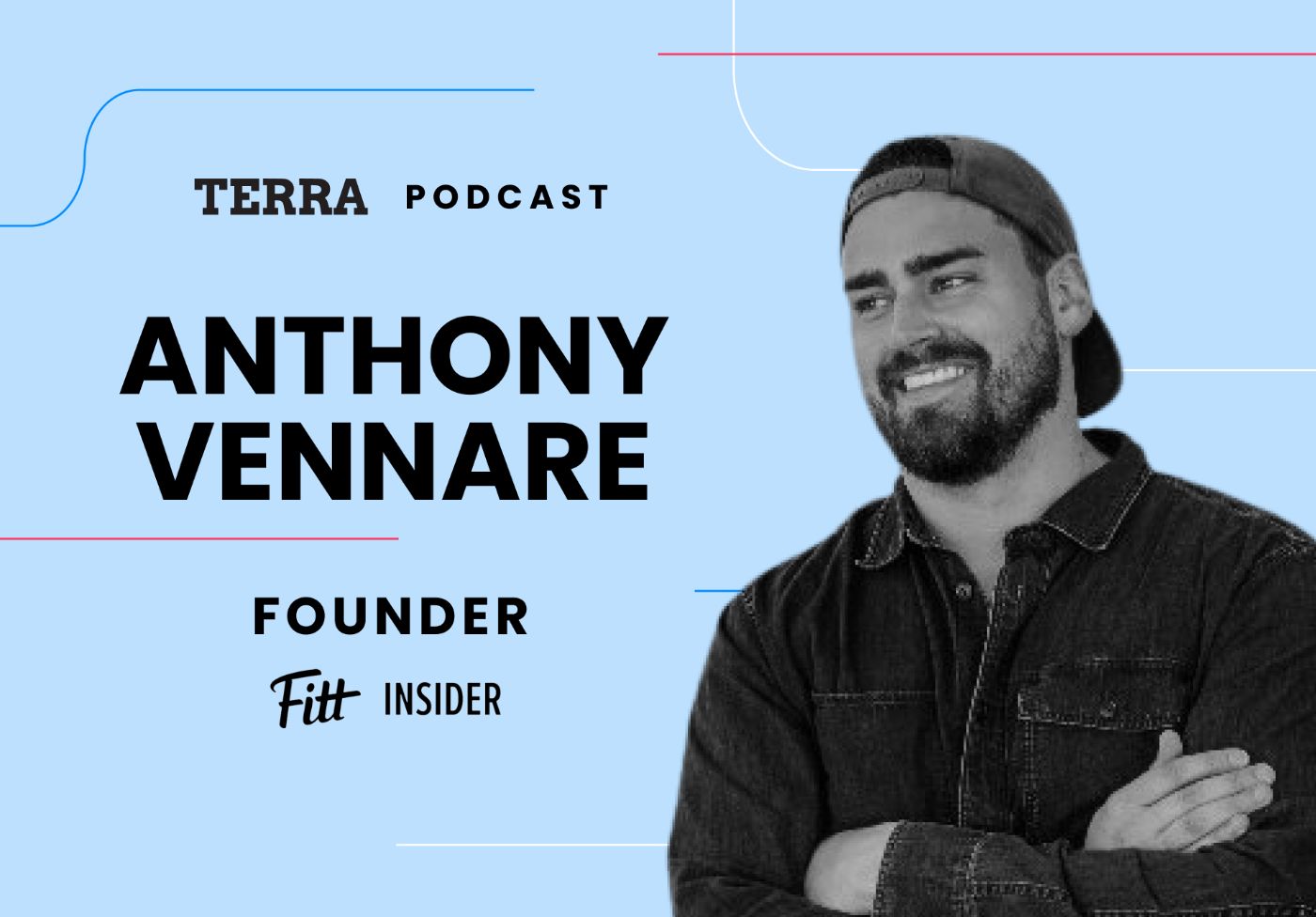 When it comes to building a successful business, the journey of Anthony Vennare, co-founder of Fitt Insider, offers invaluable insights. From leveraging persona
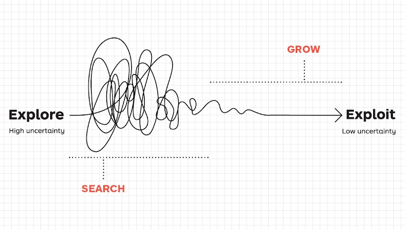 Startups need to strike a balance between seeking new opportunities and maximizing the existing ones.
 Ten stories of Ukrainian founders on leading Web3 companies during the war and bear market: relocation, working under sirens, distress, and raising capital.
 What's Your Background, and How Did That Lead You to Your Current Role?
 MeMemes is a mobile app that uses AI to transform people into over 30 famous meme images.
 How to build a start-up or product MVP without coding
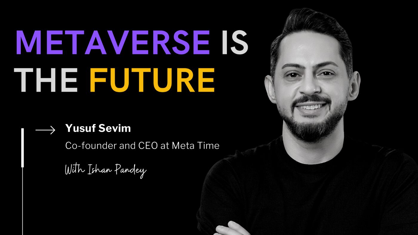 Yusuf Sevim discusses MetaTime's revolutionary journey to fuse the real and digital using cutting-edge blockchain tech, emphasizing speed and security.
 Discover how Ukrainian tech talent is driving global innovation through success stories like GitLab, Revolut, Grammarly, Wise, and Moss.
 After starting two companies, I’ve learned that sales is by far the most important skill for a founder.
 Startups usually focus on building their product first, and don’t even try to generate leads or interest until an MVP is ready. Some will just launch on ProductHunt hoping for some lead flow. But in the best case, they will get eyeballs for two days, and then no more leads come in. And building a lead flow is not that easy.
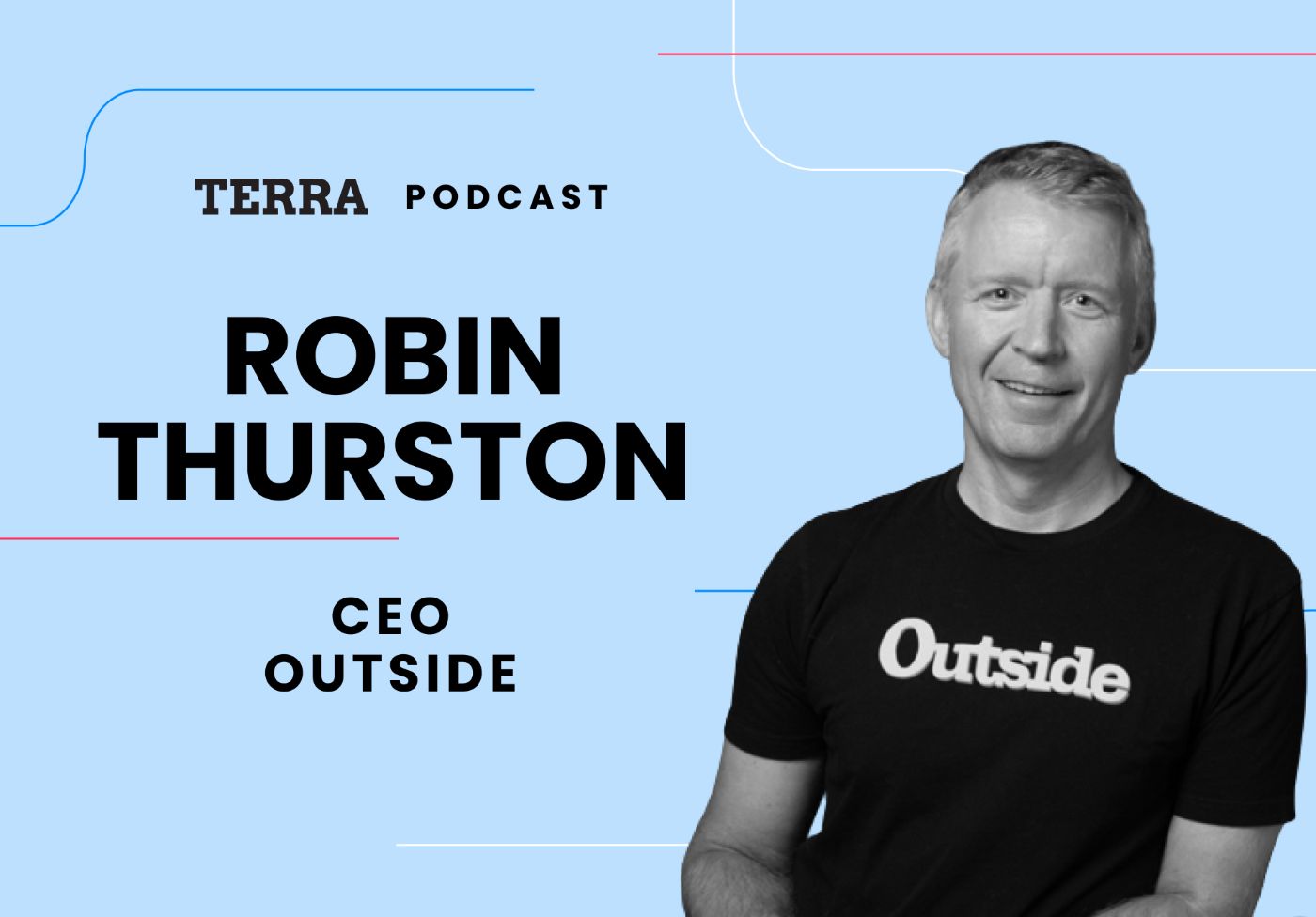 Robin Thurston, Outside CEO, shares insights: seize opportunities, prioritize customers, embrace mobile tech, build reward mechanisms, impact society.
 This is a story about how I won ‘Pioneer’ and what I learned during this program. Pioneer is a fully remote accelerator and it’s a community where entrepreneurs/indie makers help each other improve their own businesses.
 If you are a developer who is still in school or freshly (drop) out of the college or you just have a couple of years of corporate experience and have decided to take on the entrepreneurial journey as a tech-(co)founder / CTO of a startup, this series will help you understand various aspects and the role you will have to play as a technology leader for the success of your startup.
 The average consumer’s attention is now worth billions of dollars because that’s how much companies spend on their user acquisition efforts.
 The debate was deadlocked. Three members of my team at Kanary—the platform I’d built for brands to buy digital ad space—agreed with me, and three didn’t. It was 2013, and I’d spent the last year building Kanary as the company’s founder and CEO.
 Mark Gainey talks about the early challenges of creating Strava and how him and his co-founder built a healthy, profitable business.
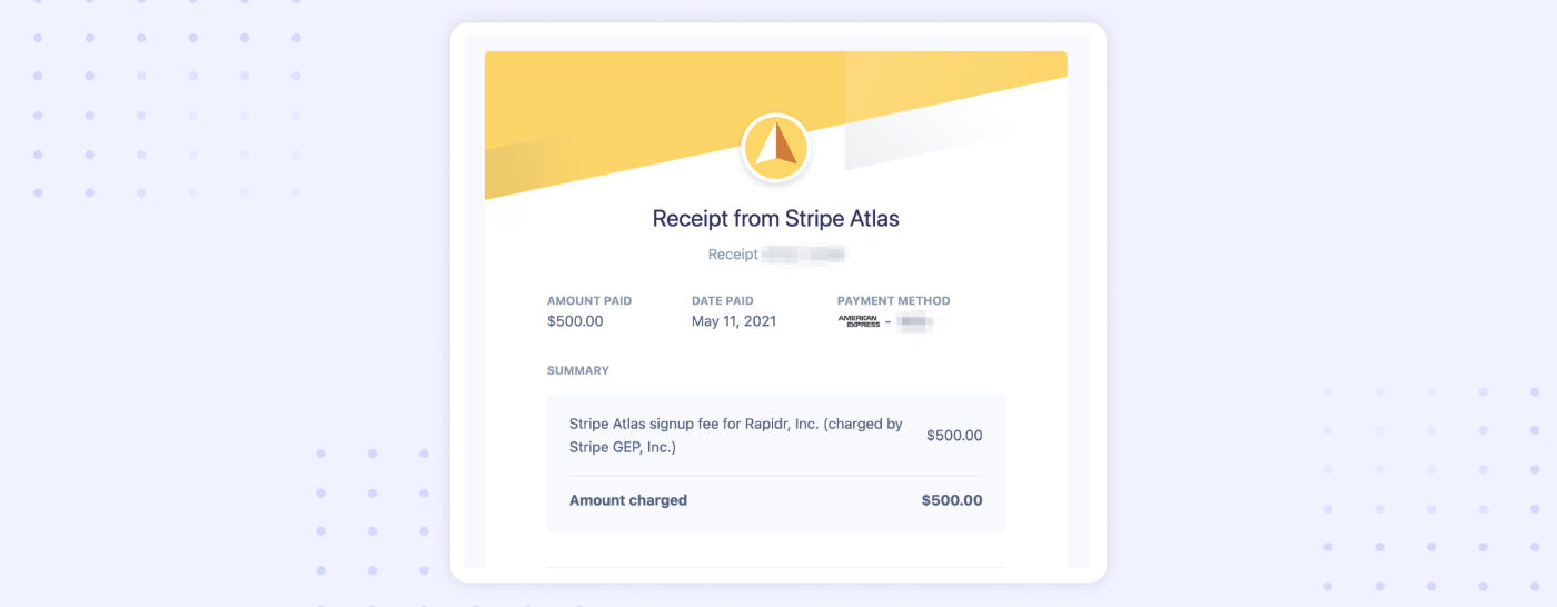 Here’s our end-to-end experience: how we incorporated Rapidr, Inc., a C-Corp with Stripe Atlas, and got set up with a business bank account, mailing address.
 In this post, you will find nine essential metrics that you should know about and measure. Your KPIs can change as your startup grows.
 Didactic's crowdfunding will change the crowdfunding space.
 This article explores the impressive achievements of these ambitious entrepreneurs and their innovative business ideas.
 Source: Zuza Gałczyńska, Unsplash
When starting your own business, it may be challenging to choose between an LLC and a Corporation. Here is some information that may make the decision a little less taxing.
 Learn fifteen+ types of projects you can turn in your next side hustle or full-time arrangement to leverage your JavaScript skills in a scalable way.
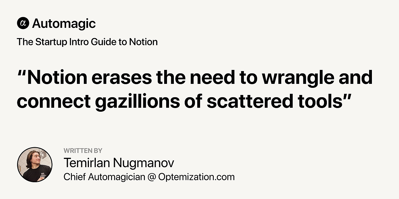 This long-form article is an informal introduction to Notion for entrepreneurs, founders and startup executives. It covers the basics and explains what makes this company truly special. It’s a 17 minute read full of film and pop culture references because why not. Also, this is my first blog post on the internet.
 Photo Credit, Giphy.com/HackerNoon, where we have 1.7M impressions since creating our account in October.
 We all from time to time come across an idea for a Startup. A company that can be a million or billion or maybe trillion-dollar worth. A company that can be next Tesla or Amazon, but sadly, 99.99999% of us don’t take the next step. That idea remains just a fragment of our memory.
 A serial founder who sold a startup to Apple and worked on infrastructure projects at Google, Harmony.one founder & CEO Stephen Tse has raised an $18M seed round and assembled one of the top engineering teams to build a next-generation high-performance blockchain protocol.
 Zoom has been in news a lot lately. It has gone from being an enterprise solution to a household name pretty fast.
 Jessica Livingston's book "Founders at work" (2007, 32 stories) inspired thousands of founders to start their startups.
 My process in building things that can invent opportunities for our business and career
 What a character. This interview began with Zoom breaking and we when we started a new Zoom call, McAfee pretended to talk without making sounds just to fuck with me. Then we hit record:
 You’re a non-technical entrepreneur and you have a business-driven vision for your startup. As an entrepreneur, you don’t need to be a technical expert. However, you do need to know the basic concepts because many tech decisions are business decisions.
 What's your background, and what are you working on?
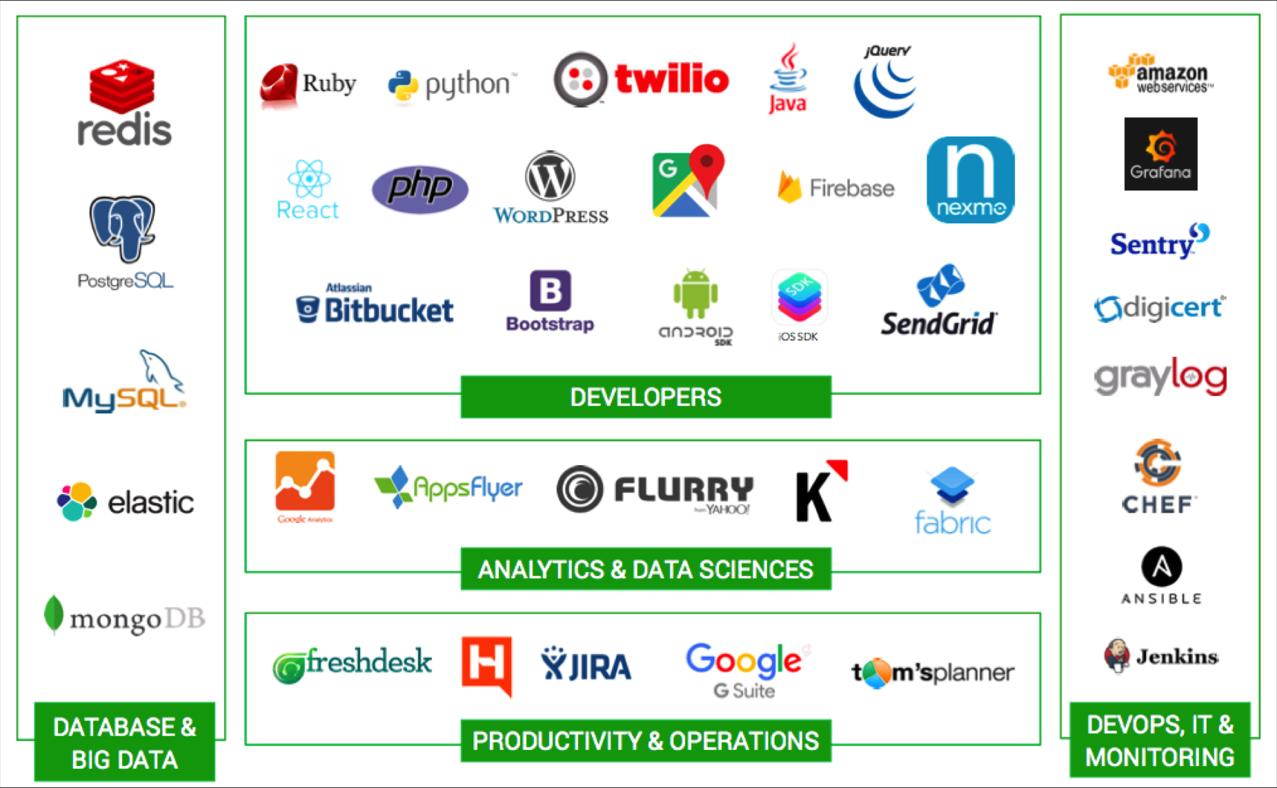
 On managing remote teams and creating an atmosphere similar to your office: Recently, I did a webinar with TIE and fellow women founders on Managing remote teams. A lot of you asked for the extensive list of tools that I mentioned in the webinar. So, here it is!
 Michael Gaizutis is the Founder of RNO1 – Experience Design Agency for Tech & Web3 Brands of the Future.
 Burnout is a scary thing. It creeps in when you least expect it. And it usually takes longer than usual for you to realize it’s even happening. Let’s back up a few months.
 More background information on the Cloud Native Testing Tool, Testkube.
 Can you remember when you used to gather in person with your team to define your roadmap and reassess your company’s collective priorities? Every quarter, our team at Pillar VC convenes for a strategic planning session to decide how we’ll invest our time and energy in the months ahead; last week, we held this meeting for the first time over Zoom. While we’ve only been working remotely for a few weeks, it feels like the world around us has changed at lightning speed.
 I sent the following note to the Sift team today. I’m also sharing it here in case it’s useful to others.
 It is hard to imagine that one small company can completely transform the way we shop. But that is exactly what Flipkart has done. In 2007, e-commerce was still considered a niche business and most Indians did their shopping offline. Internet was taking over the world and Steve Jobs had just launched the world’s first iPhone in 2007 which was about to disrupt the entire smartphone industry in the years to come.
 Bill Ottman is the co-creator and CEO of Minds, a free and open source social network with crypto rewards. They continue to make waves as an alternative to the incumbent social network business model of surveillance capitalism. Bill has also been a guest on the Joe Rogan podcast. Today, he kindly took the time to answer some questions for Hacker Noon.
 In January 2020, we met with about 45 companies. This enabled us to refine our vision (3 pivots in that month), understand our go-to-market, and start to build a list of potential clients. Once we felt confident about the product, we entered into full implementation mode.
 Welcome to the first edition of Product Stories. The first product that I have chosen is Reddit — a company that thousands of startups have tried to emulate but always failed to do so. Let’s look at why that is and what’s so special about Reddit.
 What's your background?

 So, my dear startup founders, do you know what your minions are doing while you aren't looking?
 A conversation with Joy Pathak, Evinco Winery DAO co-founder, about NFTs and how they are set to change the food and beverages industry.
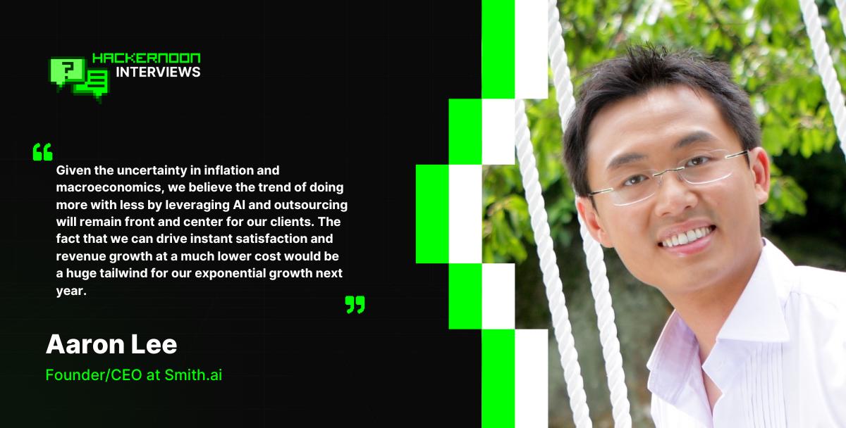 Discover how Smith.ai combines AI and human expertise to revolutionize 24/7 customer engagement for SMBs, driving growth through advanced virtual receptionists.
 What is “The White Tiger?" If you’re asking startup founders, the answer is - not just another Netflix movie, but a unique collection of great business lessons.
 The headspace of the owner is key, especially when they're hands-on in running their business, putting their all into it
 Colette Wyatt is a Chief Technology Officer at Evolve, an award-winning UK-based software house with an R&D Centre in Ukraine. She's also a Co-Founder and COO of e-bate, a revolutionary platform for rebates management, which attracted £950,000 last year from Mercia Asset Management, the MEIF Proof of Concept & Early Stage Fund, and part of the Midlands Engine Investment Fund.
 Lingke Wang and the Ethos team have recently raised over $46 million in order to simplify and modernize the archaic life insurance industry.
 Peter Kolmisoppi explains why The Pirate Bay is still alive and some websites aren't.
 The six Archetypes of Founder Madness: Imperial Individualist, Naively Confident, Strategic Contrarian, Frontier Explorer, Mad Scientist, and Global Catalyst.
 Luke Sophinos tells the story of Mark Leonard.
 Raise money without giving up a piece of your company
 Ten years after founding The Information, the tech journalist–CEO contemplates everything she wishes she’d known from the start.
 I was 24 years old. A baby.
 Please welcome our weekly sponsor Paperform to Hacker Noon! I stumbled upon Paperform when their founder Dean McPherson contributed a number of in the trenches startup founder stories, like Stop Thinking About Scaling — For Developers Working on Crazy New Startup Ideas, to Hacker Noon. Today, we’re going to catch up on the state of this startup — and find out what makes Dean & his cofounder Dionysia McPherson do what they do.
 Community commerce is transforming growth by turning customers into advocates. Learn how brands drive trust, retention, and revenue through community.
 What if startup founders learning mixed martial arts - or mixed martial arts fighters found a startup. Takeaways of traversed startup journey and sports.
 Most organizations consider customer service an overhead while it is an opportunity. It allows you to drive continued value from the customer even after a sale.
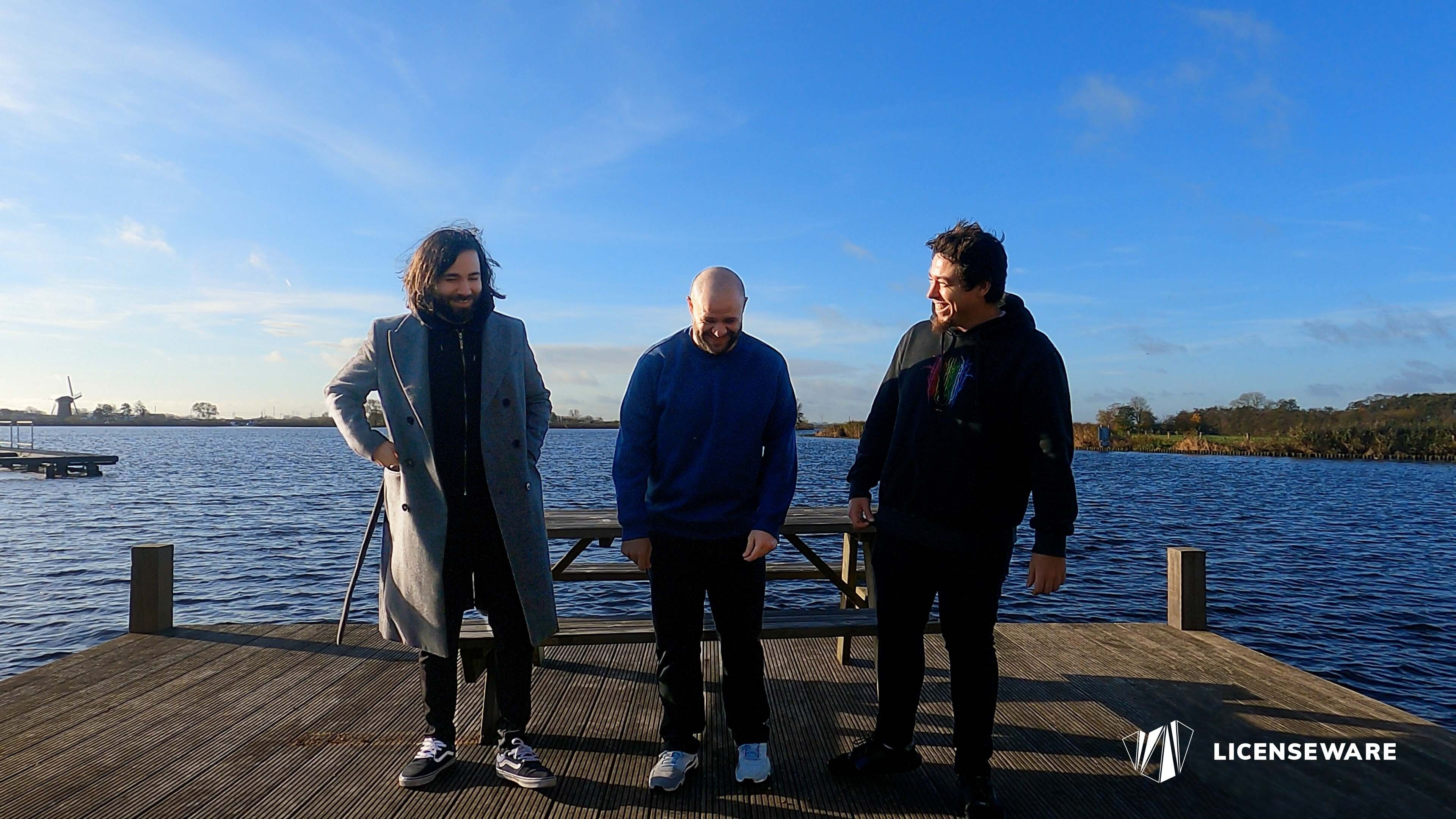 Licenseware is the first open app ecosystem for software license management. Reduce software costs and manage licensing risks, PAYIG, completely modular.
 First time founders build out of passion. They face a problem and try to solve for themselves, making assumptions that everyone has the same problem.

 Read for opinions on growing a robust community in any niche, adapting your product to the metaverse, the power of outsourcing and the future of AI.
 No-Code Report is a weekly no-code newsletter, built using no-code tools like Webflow, Airtable, and Zapier. Working at a no-code analytics firm, I wanted to learn about insights in the field more broadly, so I spoke with No-Code Report's founder, Parker Thompson, on the state of the industry and its future.
 Growth hacking once drove startup traction, but customer trust now powers sustainable growth. Learn how trust, retention, and community drive startup success.
 I am 36 years old and have long felt disconnected from the world. Not so much the natural world — that I’ve been lovingly drawn to and constantly in awe of as far back as I can remember.
 Seth Flora is the owner of LEO Digital Marketing. In his spare time, he helps founders create business plans, form strategies, and more.
 Over the past 7 years I have worked in large IT companies in the Russian Federation, EU, and in the USA. Here's what I wish I knew before I started each project
 Roughly a decade ago I decided to move away from my corporate job in investment banking in London to pursue something I always knew I wanted: to become an entrepreneur.

 Four fundraising tips from Rousseau Kazi of Threads.com
 For parents of toddlers and babies, finding the right daycare can be a huge challenge. Jessica Chang saw this as an opportunity.
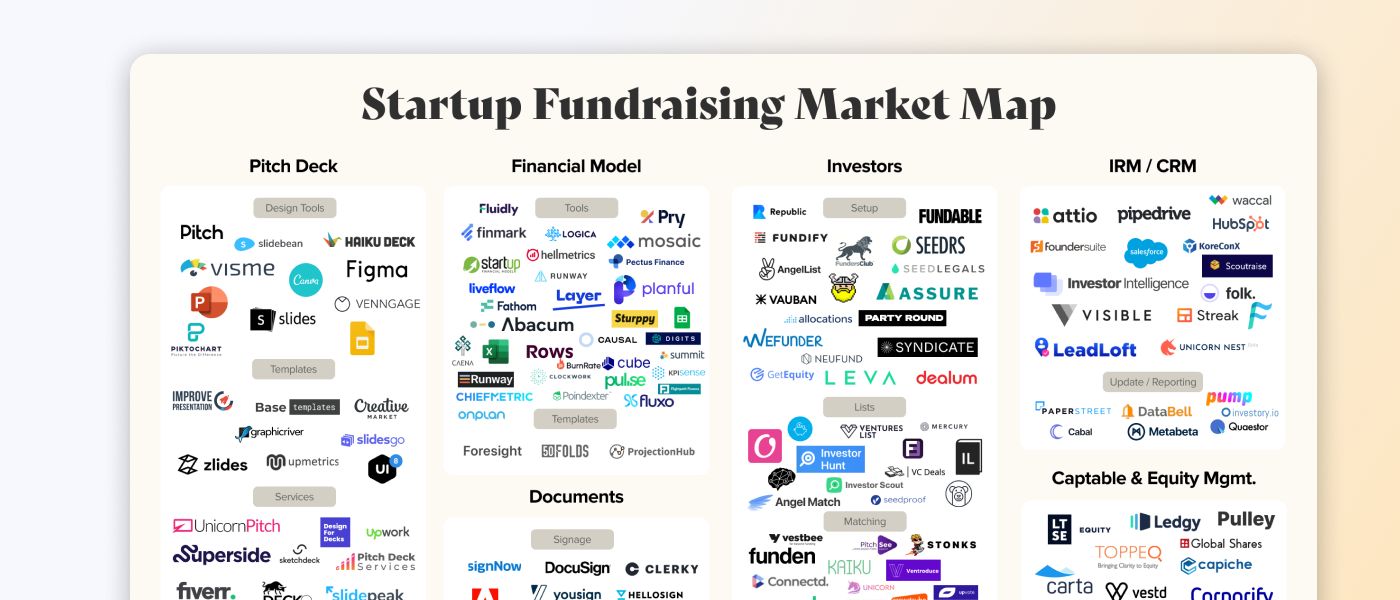 This map is a visual overview of every company that helps you get an investment for your startup, from pitch decks to captable management.


 myPluto helps small teams, young entrepreneurs and ,aspiring product managers to navigate the development of their first product in a structured manner.
 Here is how a role most people had never heard of became the career opportunity everyone's talking about.
 One of the most common frustrations among business professionals is performance metrics. Performance metrics are how employers value the contributions made by their employees and how employees clarify the expectations of their employer. It’s a simple tool that when used with intentionality can be a powerful asset for a company, but when used wrong can be one of the fastest ways to lose top talent and discourage your workforce.
 Founders and CEOs have a lot of tasks and responsibilities. Coaching the team, becoming a mentor for newcomers, and preparing for the end of the world.
 Choosing lean, scalable, and adaptable tools is the smart play.
 More than half of America’s cutting-edge companies valued at $1 billion or more were established by foreign-born founders.
 Tips and resources for applying to Y Combinator
 In this interview, we spoke to the company’s Co-CEO and Co-Founder, Ashwin Rathod about its innovation.
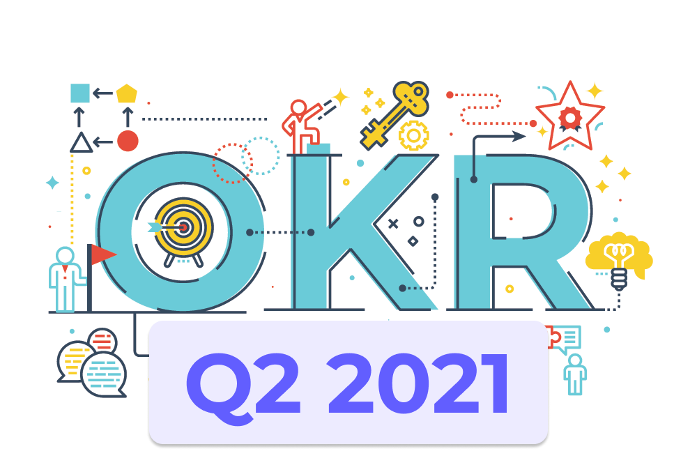 Airbyte, the open-source data integration platform, shares how they performed on their OKRs for Q1 2021, and what their new OKRs for Q2 2021 are.
 Juan Gonzalez (@Kaelon @JuanDotCo) describes how WordPress, like every founder-led enterprise, is approaching a predictably dangerous period.
 It’s been roughly two months now since the Coronavirus turned our lives upside down. From practising social distancing and getting used to a life confined within four walls. To constant washing of hands and wearing masks and other Personal Protective Equipment (PPE) just to buy a loaf of bread. All the while watching strangers, friends and loved ones getting sick, COVID-19 is truly something none of us saw coming — well besides Bill Gates.
 Anyone familiar with our project, Digitex Futures, will know that it’s been a long and eventful journey to get here. But we’ve stayed the course. Even during the worst bear market imaginable when many other projects had to throw in the towel, we’ve managed to survive.
 Startup interview with Antoni Zolciak of Aleph Zero, a public blockchain with enhanced privacy features. We combine academic excellence with business know-how.
 Pilot's annual founder survey report found that a quarter of founders are self-funding.
 March 13, 2020. I’ll remember this day as Charcoal Grey Friday in honor of my Costco sweatpants (thanks mother-in-law) and it being the hardest day of my career at GrowthHit.
 Genesis Mining CEO Marco Streng studied mathematics at the Ludwig-Maximilian University of Munich before
co-founding Genesis Mining in 2013 and becoming a passionate advocate for blockchain
technology and cryptocurrency.
Genesis Mining CEO Marco Streng studied mathematics at the Ludwig-Maximilian University of Munich before
co-founding Genesis Mining in 2013 and becoming a passionate advocate for blockchain
technology and cryptocurrency.
 If you want to start your business but don't know where to get capital, you need to find out who the investors are and why they are ready to sponsor startups.

 From raising money outside of Silicon Valley to pivoting after hitting a fundraising wall, to dealing with tornados and pandemics - Jammber founder Marcus Cobb shares his top tips for startup founders.
 Apple Entrepreneur Camp taught key lessons—app inclusivity, user-centered approach, product page optimization, app review preparation, and user rewards.
 “No” is often equated with being mean but “no” isn’t about shutting projects and people down. Here's how to say no in a corporate setting without sounding rude.
 If you’re getting your startup up and running, then you know that it takes a lot of effort and time. It also takes a lot of resources. No matter the size of the business, you are investing resources in it, and we’re not just talking about financial resources. Startup owners are also prepared to invest their time, energy, and emotions in something they truly believe in.
 Startup interview with Viktor Kochetov, CEO of Kyrrex.
 People have a wide range of different "tools" that can give them cheap and fast relief of anxiety or other psychological conditions.
 A first-time CEO shares what went right, what went wrong, and the governance mistakes every startup founder should avoid before it’s too late.
 Andrew Masanto is a two-time web3 unicorn founder, having started and popularized two of the top 100 cryptocurrencies (Hedera and Reserve).
 In this interview, we speak with Malik Drabla, the co-founder of Adrenaline - an AI project to help coders make the best of their code.
 Hacker Noon Non-Technical Founder Podcast- Episode 53 Zack Hurley

 If you’re a crypto startup dealing with stubborn institutions, you’re not alone!
 I have been speaking to Coworking spaces, Incubators and Accelerators across London and it has become apparent that there is a common problem arising from non-technical startup founders. This transcends the culture, this impacts more than just female or minority-led startups.

 A few years ago, Matthew Klein and his brother Andrew saw that the retail landscape was changing and that companies needed more agility than ever.
 My "Tough Love" Talk To Founders Who Are Struggling To Raise Capital
 Bringing Dishonest Crypto Journalists Lies to Light - The Story of Danny De Hek and Sultan KassamBringing Dishonest Crypto Journalists Lies to Light - The Story
 Eowyn emphasizes security in the crypto realm amidst rising cybersecurity threats.
 Marc Randolph goes over the importance of building a great team.
 The cryptomarket is melting. The cryptomarket meltdown is a result of the bearish sentiment in the market.
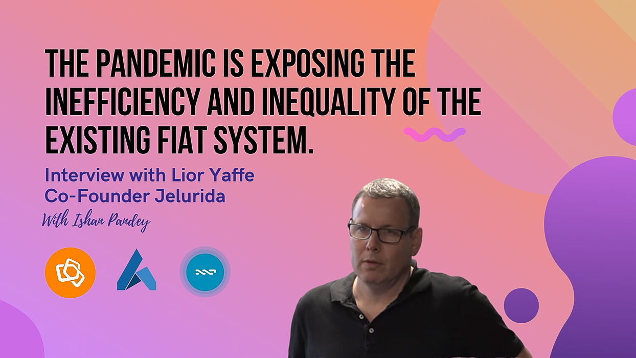 "What I see is how the pandemic is exposing the inefficiency and inequality of the existing fiat system. Governments are printing money to bailout those who recklessly spent it during the good years. Banks lending government-backed money to those who don't need it instead of helping businesses in distress." - Lior Yaffe, Co-Founder, Jelrurida
 Childhood friends James and Allen are making it easier for companies to build machine learning teams with AdaptiLab (Techstars Seattle ‘19).
 You’re going to spend more time with your co-founder than with your spouse. This is why finding the right one is the one activity you CANNOT afford to rush. If you’re truly passionate about founding a company, you have only two options: compromise or keep on looking.
 Serial entrepreneur Andrew Hoag had a huge frustration.
 There are a number of prominent startup examples that have been very successful in the past few decades like Facebook, Instagram, and Airbnb among others. But from these stories of success, quite a number of failure stories are left untouched. According to an estimate 9 out of 10 startups end up failing. Entrepreneurs publish post mortem online and they are quite haunting. The reasons for failure may depend upon various factors like insufficient funding, incompetent team, and lack of motivation. I have compiled a list of 10 reasons which have been the cause of startup failures.
 How building in public helped the growth of my startup.
 What's your background, and what are you working on?
 For most companies, growth marketing is the way of the future for leveraging data and agility to scale revenue and increase customer lifetime value.
 Matt is the co-founder & VP of Marketing and Developer Relations at Manifold, the cloud-native marketplace company.
 Why I left Google to found an AI startup funded by Techstars and Peter Thiel.
 Despite the bear market startups should not turn off their projects in the crypto industry and Web 3.0. A few tips for projects on how to start in a bear market
 The concepts behind Erlang/OTP/Elixir make it a great fit for a tool like the one I was building
 I think the ICO run is past us. We will not see a crazy market like we did in 2017. Scammers are very sophisticated and are always coming up with new ways to scam.
 True to my conviction that blockchain's enormous disruptive potential can change the status quo, I recently sat down with Bolaji to explore AgriFi and Tórónet
 The world of AI startups is rapidly expanding, with a multitude of new players and innovative solutions in various industries.
 A conversation with Jet Liu on how a combination of AI, Web3, and innovations in computation technology can help shape the future.
 Choosing the right set of frameworks, database, front-end tools, back-end tools to build a long lasting tech stack for your SaaS
 On the Importance of Building Healthy Co-Founder Relationships, Navigating Investor Meetings, and Investing in Your Mental Health as a Founder.
 Daniel Quoc Dung Huynh, CEO and Co-founder of Mithril Security, is launching a startup to democratize privacy-by-design AI tools.
 10 Lessons I learned after making $1K as an Indie Hacker
 We all have different roles to fulfill during a product’s journey. Some of us are heavily invested on the sales and marketing side while others consider the technical decisions as their day to day job. While segregation of work is important as well as useful for founders, there are a lot of things that all founders need to learn to make sure they are ahead on the curve as they take continuous decisions for the product and its growth. Here are 10 things to do right away as you start your product journey.
 When it comes to selecting the right back-end technology. It can be confusing to evaluate your project needs and a versatile fit for your back-end development. However, NodeJS can be the best fit for your product. Thus, hire NodeJS developers to build the best business solution. Some of the crucial factors include whether you should look for offshore or onshore hiring.
 You have built a tech startup to provide an outstanding solution, but it is not necessary that all the people will understand your idea in the beginning.
 Yes, we’re witnessing a crisis unfolding. Not only people get gripped by the coronavirus fear. It’s like a stroke for most businesses — some will recover, some won’t.
 With a new political wind blowing through Brazil, we need to ask: What impact might Lula's election have on the buzzing startup ecosystem?

 It is important to realize that we have the ability to manufacture our own fate when we want to. - Eric Haney, Delta Force operator
 I’ve been a full-time founder for almost a year but have been into startup culture for most of my professional career as a software engineer (~4 years).

 Unsuccessful startups are all alike; every successful startup has succeeded in its own way.
 Software Development is a route that’s proved to be very popular in the last couple of years in tech. From HTML & CSS webinars to Ruby on Rails meet ups, you can’t escape the hype. But what if coding isn’t for you? What if you want to solve problems in Tech without writing code, is there a career out there for you?
 Anti Danilevski, KickEX CEO and founder, talks about Top 5 Methods of Running an Effective Cryptocurrency Exchange based on his own experiences in the field.
 What's your background, and what are you working on?
 Geoffrey Frank is the founder of Myntist, a startup that combines e-commerce and d-commerce platforms into a digital hybrid ecosystem.
 In July, my brother and I launched our first software product after nearly 2 years of working full-time on our business. We hit a big milestone that month and generated our first $10 in software revenue.
 Lose the to-do list, there is only one thing you need to focus on
 A new breed of tech visionaries has been instrumental in driving this change and helping to deliver Web 3.0 solutions to the masses.
Explore Sound.me's journey, an AI-driven influencer platform transforming influencer marketing with simplicity, accountability, and global reach.
 I’ve always found naming things to be particularly challenging. That is because a bad name is way worse than a good name is good - naming your car the “No-Go” (as the Chevy Nova was in Spanish) is far worse than a decent name like the Passat is good. Naming is, unfortunately, a negative sum game.
 David Sutter is the CEO of OpenTrade, an institutional lending platform that provides users access to a suite of on-chain credit products for tokenized real-wor
 I know what you’re thinking. “That title has to be a typo. No one could grow that fast!”. I’m here to tell you that if you work hard and pursue your dreams you too can make $10 in 2 years.
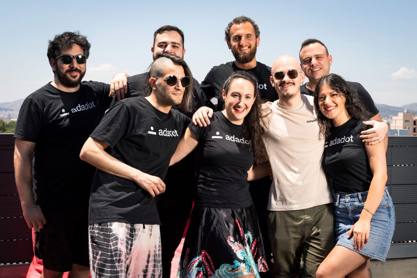 I’m Alex and I’m the Founder at Adadot.
 I am speaking with James Wo, the CEO and founder of the investment firm Digital Finance Group, to discuss promising sectors within Web 3.0 for investment.
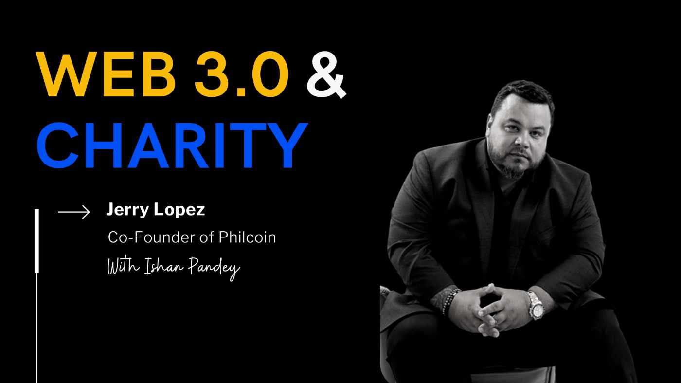 Philcoin is the world’s first philanthropic blockchain super dApp, says founder Jerry Lopez.
 That are countless blog posts that extoll the benefits and power of digital marketing. There are even more that show you exactly how to do it.
 To start with, this is a tricky topic, where I might find people in conflict with my perception but after all when isn’t conflict a promising act. Conflict by its meaning is a disagreement where one holds an entirely opposite perspective and surely does one defend it as if it was their very own life at stake. I think that is a beauty of it, perhaps lasting for a long time that is unexpected or usual. I would put it as my experience to suggest that I have seen people get excited and enthusiastic about doing something. It can be an idea or a project or anything that they either want to achieve in life or a common goal to which one puts an effort.
 Learn from our twist-filled journey and gain valuable insights. Find inspiration and guidance for your own pivotal path
 A short story of a workaholic engineer switching from a developer to a product founder in 10 years.
 Let's make the business world beautiful with brand designs.
 Explore Patrick Brown's vision for Unity Communications, blending superior BPO services with his love for DJing.
 Remote work is booming largely because of the lockdown. But this way of working has been around for a long time - especially among knowledge workers. During the pandemic, a lot of companies tested remote working for the first time, and most of them do not plan to go back to the office even after the lockdown. However, some holes need to be patched and things taken care of before any founder jumps into remote working permanently.
 Lessons from a founder on shaping startup culture that scales — from hiring and leadership to trust, transparency, and building a team you’re proud of.

 In the beginning of June 2020, we had enough cash to sustain ourselves for 2 years, and had decided to pivot. At the time, we weren’t sure if we needed to move away from our product, on which revenues were growing very slowly, or not. We spent 6 weeks in full exploration mode to identify what our next step was.
 Are you a startup founder? Consider filling out these writing prompts so readers can get to know your company better, and it's a great way for others to learn.
 Never underestimate the power of sharing what you think. Write, publish, post. Technology is built that way — brick by brick, idea by idea.
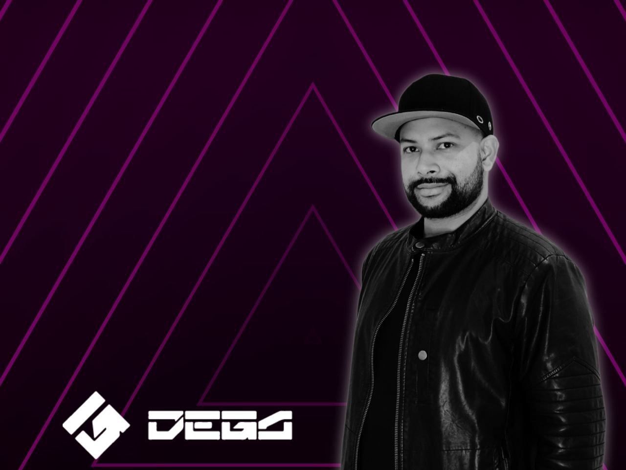 In this interview, you are going to learn more about Carlos's blockchain career and DEGA, his brainchild.
 Timeless advice to profit from your passions, capitalize on your ideas and become a better human being.
 5 reasons why you should do competitive analysis before building a product ?
Using competitive analysis, startup founders can get a head on in product.
5 reasons why you should do competitive analysis before building a product ?
Using competitive analysis, startup founders can get a head on in product.
 One thing that has become clear in the last few years is that the soft parts of data science are becoming even more important. What do I mean by soft parts? I a
 Achieving a €260,000 with My Central European Software Engineering Leadership Venture.
 Nicole Nguyen is the co-founder of Duelist King, the first NFT game powered by Dual Launch via OccamRazer IDO and PancakeSwap IFO.
 Forter is the leading provider in e-commerce fraud prevention, protecting $130B in digital transactions annually.
 Miki Agrawal shares her most thoughtful and inspirational quotes about life, entrepreneurship, technology, and not letting the haters win.
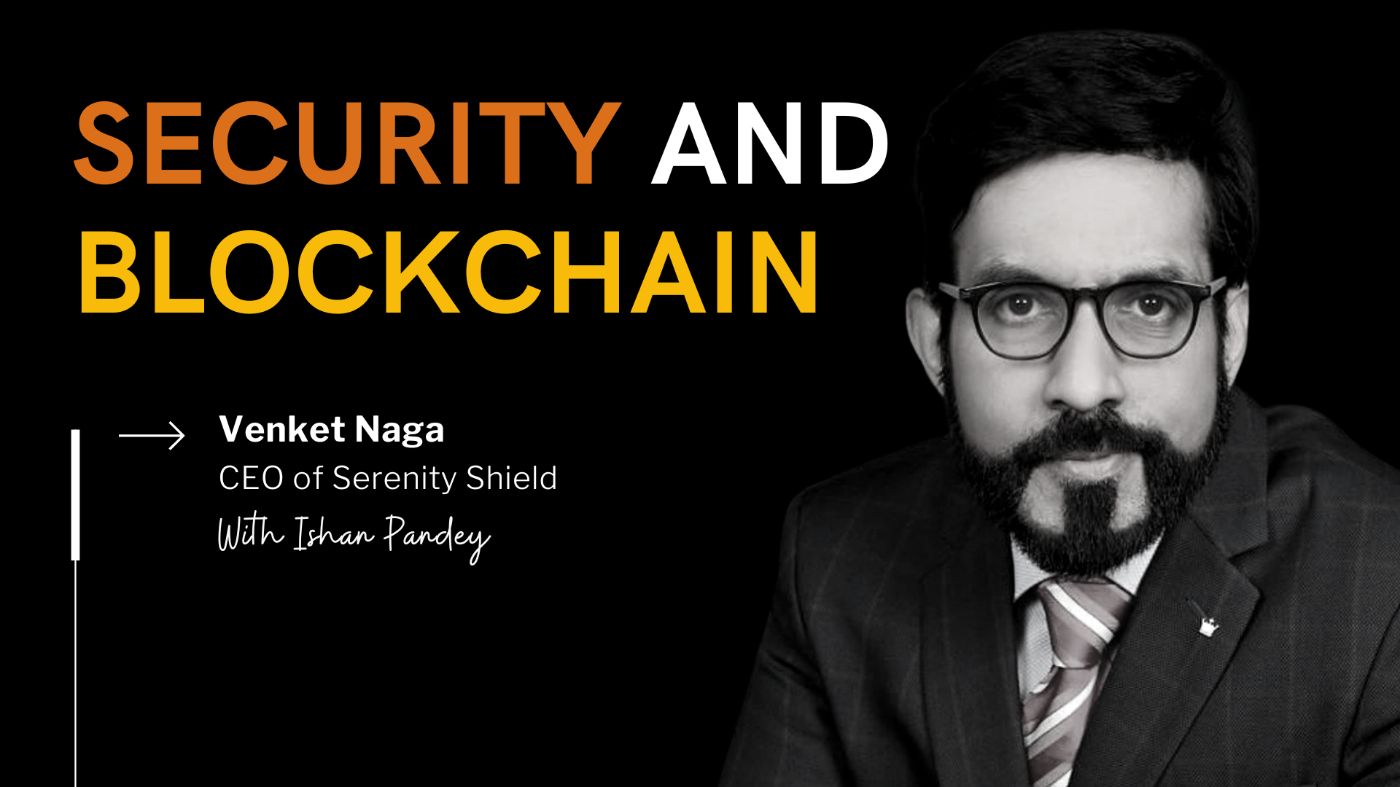 Venket Naga, CEO of Serenity Shield, talks about his journey in tech, the inspiration behind the blockchain initiative and how it aims to redefine data security
 Adam Knuckey, co-founder of Dolomite, shares the story of its inception, the challenges faced, and the vision for the future.
 Every decision and step we take at a startup is based on some belief. Here's how to validate those beliefs and build products like a scientist ;)
 Estimated Reading Time: 14 minutes
 On this episode. Jon Dahl, CEO of Mux, and Thierry Schellenbach, CEO of Stream, talk to Amy Tom about starting their API-powered platform.
 In this interview, we catch up with Zachari Saltmer, Co-Founder of One Big Fund to discuss the state of VC funding, AI, and crypto.
 Why untested ideas remain illusions. Only through simplicity, speed, and real-world testing can you separate what’s real from what’s not.
 Sowemo Tech Private Limited Founded by Ketan Shrivastava and Surendra yadav in July 2019. Basically its a IT service company located in heart of India at Bhopal Madhya Pradesh. Its a long journey travelled by Ketan from 2012 When Ketan was in final year of engineering in 2012. He had idea of Talent Search Portal. At that time in Bhopal Engineering students have potentials But was not much aware about Angel investors.
 Levin shares his views on hiring remote tech talent, the benefits and challenges of remote hiring, and strategies for finding and retaining remote talent.
 A couple years ago I was teaching a small course at Stanford about Entrepreneurship and I remember the number one question was how to raise money.
 Find out what you need to do as a co-founder during product development when you have little to do but still need to contribute to the success of the startup.
 I had the chance to talk to the Facebook Video Expert Dalip Celbeqiri who is the "go-to-person" when it comes to creative marketing. You can catch him behind the scenes, usually brainstorming and creating master plans for viral content. Dalip is one of the founders and CEO for the company Following Media Inc. His team runs the marketing for some of the biggest brands like “DIY Simple“. His team currently holds the 2nd place for “most views on a Facebook video” with more than 4.5 billion minutes viewed in a year; 100% organically.
 Surveys suggest that over a third of the world’s female entrepreneurs have experienced gender bias. Only about 6.4% companies have women CEOs.
 7/22/2023: Top 5 stories on the Hackernoon homepage!

 The title of CEO/Founder seems cool but it's all about burning our hands and heads by Hustling. It's not like a general race where once you run quick and finish before anyone else and win the game. To be honest, entrepreneurship is like slowly moving with high efforts for success.

 Jack Altman, CEO of Lattice, goes over first-time founder misconceptions.
 AdValorem Angel Syndicate drives the future with investment in machine learning.
 After scouring the internet and tapping into whatever it is I've learned about building teams and leveling up the purpose of work, I came up with 20 questions for the Hacker Noon team to reflect on the year behind and improve for the year ahead. Maybe they can help your startup or team too? So, I'm publishing them here.
 Here's how to look for investors on LinkedIn, and what should be in the first email to get interested in your project.
 After the announcement and news on raising our first external round of capital, several budding African entrepreneurs have reached out to me through various social media channels asking, "Tesh, please could you share some tips on how you did it?" Reflecting upon the same and the numerous congratulatory messages that came streaming in this past week made me think about the struggle of fundraising, and why it is indeed a great milestone for entrepreneurs. As much as the capital we have raised ($350k) for our startup, MarketForce 360, is very 'small' - compared to some counterparts across the globe - I have come to learn that less than 0.5% of startups globally get funded by either angel investors or VC's (venture capitalists). In Africa, the statistics are worse!
 Discover why app-hopping is a productivity killer and how Unified Niche Ecosystems reclaim 59 mins/day lost to digital fragmentation and Micro-SaaS failure.
After scouring the internet and tapping into whatever is I've learned about building teams and leveling up the purpose of work, I came up with 20 questions for the Hacker Noon team to reflect on the year behind and improve for the year ahead. Maybe they can help your startup or team too? So, I'm publishing them here.
 Recently I had a chance to chat with Adel de Meyer, entrepreneur and leader of DAPS coin, a fully anonymous staking coin and payment system. Her project recently published a new DAPS whitepaper and announced its web wallet.
 Here's a big list of things that don't seem to work, based on the last 20 years of running Tiny:
 I've been working in technology for the last 17 years, and I cannot help but admit that — as rewarding as this industry seems — it's a never-ending race with time, and the speed at which the disruptive becomes outdated is unparalleled.
 The Black in Tech Interview with Emmanuel Nwaka.
 Stewart Kohl is Co-Chief Executive Officer of The Riverside Company, a global private equity firm based in Cleveland, Ohio with offices across North America, Europe and the Asia-Pacific region. The Riverside Company has more than $7 billion in assets under management and oversees a global portfolio of more than 80 companies. Prior to joining Riverside in 1993, Kohl served as vice president of Citicorp Venture Capital and COO of the National Cooperative Business Association in Washington, D.C
 As a kid I always wanted to be the best at what I did: school, sports, games, you name it. I remember playing cards with friends and if I lost and somebody laughed, I would get very upset and disappointed.
 Today, I am talking with Leo Nilsson, co-founder of a mobile chat app - Scapin'. Scapin' is designed for our virtual identities.
 Jamie I.F., Founder of AffiliateFinder.ai on Helping SaaS Teams Automate Affiliate Recruitment and Grow Faster
 Maxim Lukyanov shares insights on how business developers and high tech companies attain noteworthy results through the secret and power of networking
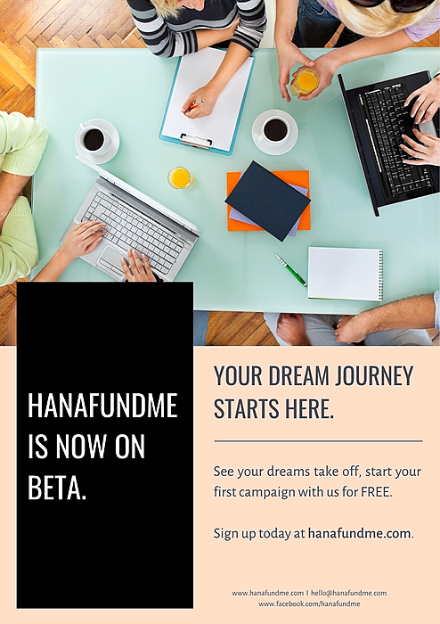 Starting up business, if you are cash strapped, can be pretty tough. It is still workable, but the journey is longer. Having extra funds helps you sustain your business operations and makes it easier to scale for growth.
 I've often fantasized about time traveling to coach my younger self. This is the advice I'd give myself when I was launching my last startup.
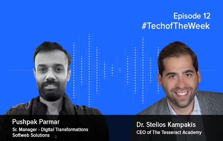 The blockchain is a distributed ledger that records transactions in a permanent and verifiable way.
 Let's be honest, starting a business can be challenging, but for many people (like me) - it's a lifelong dream. Although many people feel more comfortable starting a business with a co-founder - it's not always the best decision.
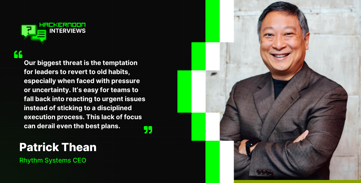 Patrick Thean is an award-winning serial entrepreneur who has started and exited multiple companies.
 PDF API, fill, generate and e-sign PDFs
 Recently we decided to start trying harder to market our side project, Notifier.so - Get Notified when your business is mentioned on Reddit and more, and as part of that process we submitted it to a bunch of directory sites we found in an older article.
 Here are some top dos and don'ts for startup founders, alongside some management tips for startup founders from successful entrepreneurs.
 Why will more people switch to cars as their choice of transportation? When will all vehicles become self-driving? I had the opportunity to sit down and talk about these issues in greater detail with Alexander Sapov, the CEO of GetTransfer.com, one of the biggest airport-to-city transfer providers.
 A story on wellness retreats and their benefits in today's digital age. How technology takes a toll on us and what to do about it.
 While Debbie Wei Mullin was fundraising for her specialty Asian beverage company, Copper Cow Coffee, she encountered frequent skepticism about its appeal: “it’s a niche product.”
 Who doesn’t know Panda Express? It is a fast-food restaurant chain that offers American Chinese cuisine. With over 2,200 locations, it is a forward-runner in the Asian restaurant chain niche. The idea of Panda Express was born in the United States. First restaurants used to be located in shopping mall food courts, but the chain has been expanded since then. You can see Panda Express in universities, airports, military bases, amusement parks, and other places.
 After years of running events for huge companies, Allie Magyar decided she was spending too much of her time hovering over a fax machine.
 Lomit Patel, Chief Growth Officer at Tynker, provides an overview of the pros and cons when building or buying an AI martech solution to capitlise on growth.
 Often, the problem lies not in hasty or incorrect hiring decisions but rather in the failure to correct a wrong decision promptly.
 Feelin | Share what you feel
 Why you have to own your process from end-to-end
 Interview with Tyler Hochman, CEO of FORE Enterprise.
 A self-starting entrepreneur with 13 years of experience in HR managing, Hyunkeun Yoon. SOMESING is another Blockchain project, which recently won at the Blockbattle Korea 2.
 Sarah Mei goes over Richard Stallman.
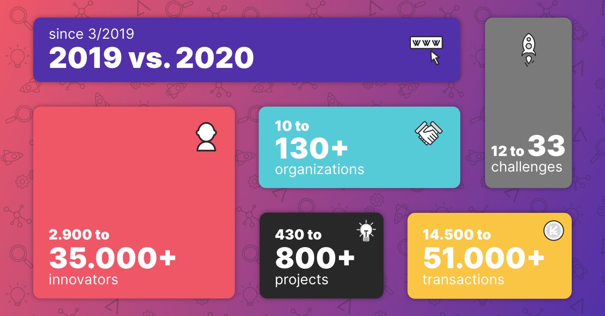 Year Highlights for TAIKAI's Product, Community and Challenges.
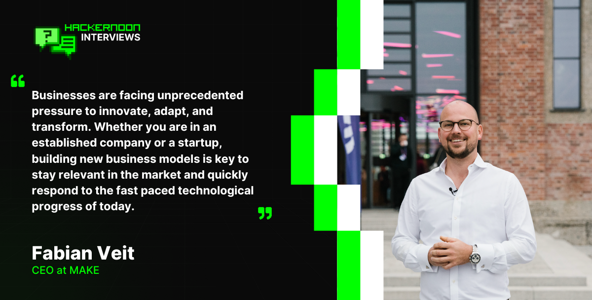 Discover how MAKE Founder & CEO Fabian Veit drives innovation with visual no-code automation, empowering businesses to adapt, innovate, and outpace competition.
 Emizentech is recognized as one of the trending startups in Jaipur India in 2022 by Hackernoon.
 Embark on an entrepreneurial journey while maintaining balance in health, finance, relationships, and spirituality. Thrive in all aspects of life! 🚀🌟
 A recent nationwide survey aiming to better understand the “before and after” of emotions in relation to the COVID-19 pandemic has found that people’s #1 emotion now is anxiety, and before the outbreak, the #1 emotion was calm.
 How to build successful companies and what tech leader should look like in the AI era?
 In this exclusive interview, Brunk delved into the origin of DTrust, the benefits and risks associated with smart contract-based trusts
 I quit my job. I'm now unemployed. It feels great to finally be able to write this blog post.
 Your home life isn't separate from your business. It's the foundation everything else is built on.
 Don’t aim to ‘become a thought leader’. It’s not about the label. But do strive to make a difference in your industry with thought leadership.
 The article gives you an idea of how the top SaaS companies made progress and ranked themselves in the top list.
 TLDR: See mozilla.org/builders for more details regarding our summer programs!
 The millennials are too tired of 9 to 5 jobs and a monotonous lifestyle for a decade now. They have a good skill set and corporate experience, which pushes, them to open startups with the knowledge gained from their work environment. But does everyone see success in venturing startups, and what are the difficulties they face to be consistent in their entrepreneurial dreams? Let us see the top 10 reasons for tech startups fail and how we can recover and be ready with measures to overcome the failures:
 When the travel industry will recover after the pandemic, what will the travel experience look like and how modern tech will influence it?
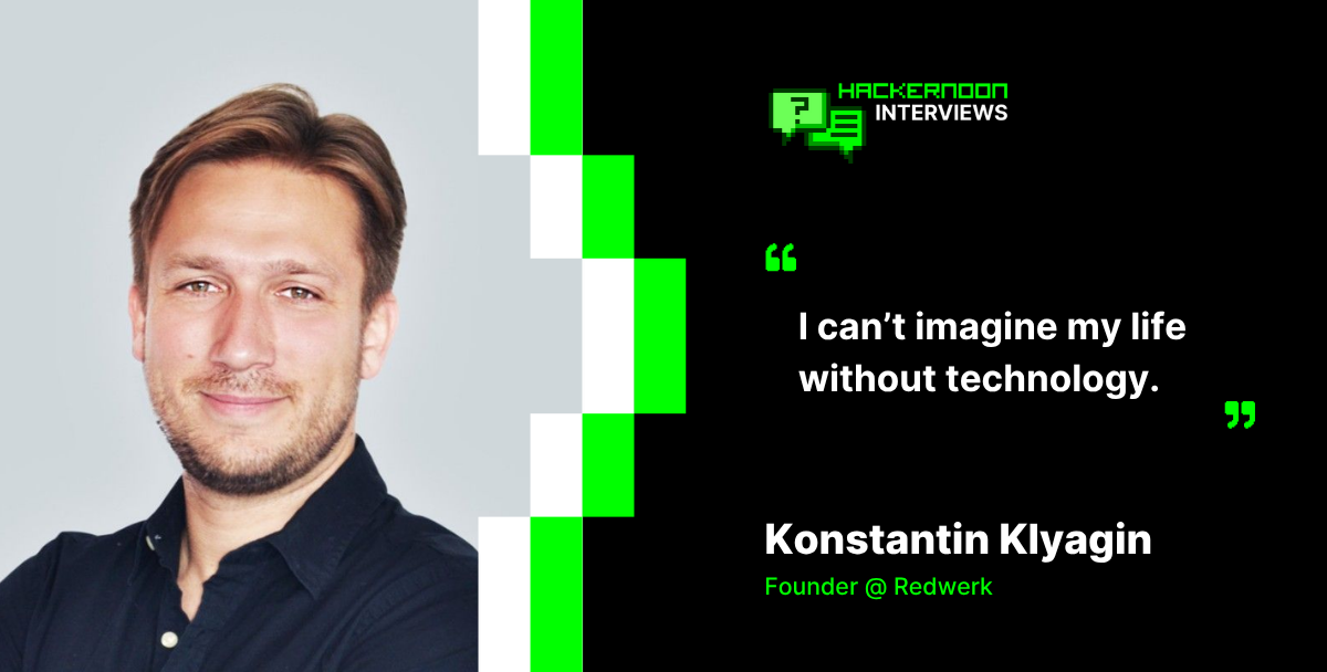 Redwerk’s Founder shares how the company became a trusted tech partner for Fortune 500s, serving 773M users through custom software and digital transformation.
 A text editor where Pac-Man will start eating the text whenever you press backspace.
 Iteration is the new innovation…
 When product scale outpaces narrative clarity, teams accumulate narrative debt. A systems view of why growth quietly breaks alignment first.
 Building a successful WEB3 startup is more like trying to navigate a maze blindfolded while riding a unicycle and fighting wild feral hogs, but you can do it!
 This article will show you 4 tactics for optimizing your SaaS sales funnel
 No, seriously, why not? It’s cool to be a designer, a creative person who DJs vinyl sets in a funky club at night and starts the morning with a double-filter coffee and a vegan croissant overlooking the sea to get inspired for the next advertising campaign. Not a bad stereotype, right?

 Founder dependence isn’t just an operational bottleneck, it’s a risk multiplier that will kill any operator's chance of exiting a business.
 Carina Ayden, the founder of Unimaginable foods, shares her perspective on the sustainable lifestyle and becoming an environmentalist.
 Advanced systems are scaling faster than markets can interpret them.
 CulturePulse's fearless female co-founder and CPO pushes the boundaries of product development in AI.
 After the uncertainty of the year 2020, we have to admit: the new order came up from the chaos, and as a result, the business priorities were reconfigured too.
 Starting a business is hard and requires making tough decisions. More than that, most startups struggle to find the necessary investment. This is why many startup founders seek to join an accelerator that will make the initial investment and provide quality mentor support.
 Hacker Noon—where hackers start their afternoons, has partnered with Stream to present the first inaugural Noonies 2019: The Tech Industry's Greenest Awards. You can help Hacker Noon declare the best and worst of this year's tech scene by voting every day from today until August 16th!
 Miki Agrawal champions ongoing global sustainability and eco-friendly hygiene through her professional and personal life.
 By a deep study into the market systems before launch, the company pointed out shortcomings within the crypto industry.
 The only way to learn is by starting and doing things relentlessly. You should go deep into a chosen space, and don't worry about making big leaps.
 Are you being the best leader you can be? Is your leader effective? here are some useful tips on how to do better.
 Muhammad Bilal (Pakistan) is a 5x 2020 Noonie Nominee for contributions to the Entrepreneurship, Founders, IoT, Life, and Life Lessons tag categories on Hacker Noon. In this interview, Muhammad shares personal perspectives regarding self-awareness, problem solving, and stagnation.
 Sam Blond discusses founder-led sales.
 My name is Omer, I am the CTO and Co-Founder of Swimm, a devtool that helps developers and their teams manage knowledge about their codebase.
 It might just be a sign of the times, and it definitely feels like so much has been said about DeFi already.
 College is a great place, you make new friends, try new things, and have no shortage of homework. During my freshman year at Iowa State, aside from doing normal college things, I spent my time learning as much as possible about how people have made technology solve problems for society and everything that goes into making these ideas a reality.
 Cybersecurity is often cited as a minefield for businesses, and while this cliche remains true, it has become slightly outdated.
 If you are aware of the values of carrying out the Product Design Process, then you are halfway through the success!
 A cautionary tale of ambition, denial, and the costly consequences of building a startup without a clear problem to solve or customers to serve.
 To start your own business or a startup you don’t need to have a degree in business specialization or business experience. All you need is to know how business works and do proper business planning.
 It was a big, scary decision to make—going from a conventional 9-to-5 desk job working in operations of a small company, to launching my own digital business where I work as a content manager and writer.
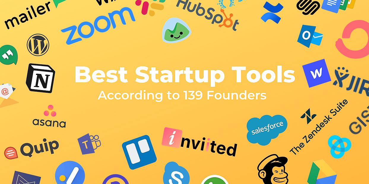 As Startups, we have a habit of moving fast. But in our haste, did we pick the right tools for the job?
Founder Nicky Watson shares insight into her company, Cassie, with HackerNoon's '10 Questions for Every Startup Founder' interview template.
 Analyzing how successful indie businesses are able to differentiate themselves.
 Roy Simmons coined that phrase and I like it a lot. “Most artists can’t draw.”

 George Thomas McCormick is the founder of SOAR: a full-funnel Facebook & Instagram marketing agency. SOAR's main offering is creating and running profitable Facebook and Instagram ad campaigns for its clients.
 22-year old Founder of ThePeer, Michael Trojan Okoh, shares his story with me.
 Valuable Lessons learned from 5 successful public building founders.
 A strategic framework for hiring high-potential talent — even if they lack experience. Based on real-life practice, behavioral psychology, and experience.
 Dominik Tomicevic, founder and CEO of Memgraph answers ten questions for startup founders from HackerNoon Founder and CEO David Smooke.
 Learn everything you need to know about Davis Baer via these 7 free HackerNoon stories.
 It is common advice for founders to build only things they are passionate about. But, there's another side to that story.
 This year, applicants to the Greater Colorado Pitch Series can apply for 4 different capital tracks and $1.3M in total investment is available.
 It looks like progress, it feels like progress. But nothing ships. This is avoidance in a very nice hoodie.
 The many pivots of building a startup from a UK Founder
 Interview with Marianna Alshina, CBDO at Know Your Dosh for Hackernoon.
 The fastest way to build predictable, sustainable growth is learning which signals deserve your focus and which are just noise.
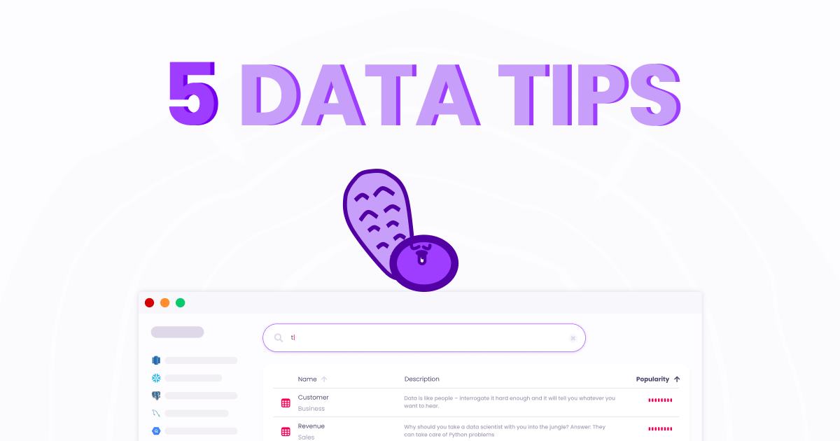 The 5 things every data analyst should know and why it is not Python, nor SQL
 Wonder has one key concept and it is that “the future is collaborative”
 Join us as we sit down with Jay, the Co-Founder of Genopets, as he shares his journey in building a blockchain-powered gaming platform and the insights he gaine
 As you prepare for your board meetings, you might be struggling to find some good news to share with the board. Sure, it’s a mistake to go into a board meeting pretending everything is going well — board meetings are a valuable opportunity to share your startup’s challenges and get guidance from a panel of trusted advisors.
 We spoke to Jason Hines, the Co-founder of Gigasheet, a big data spreadsheet platform…
 The ongoing pandemic has impacted not only our lives but also the global economy. COVID-19 will stay with us for months to come and it is unlikely that our world will ever look the same. This is the time to adapt.
 Arengu was officially founded in May 2018, but we had to come a long way before finding our value as a company. Today, we'd like to share our road with you, so you can get inspired and learn from our story.
 Fear of missing out
 I’ll not deny it. I love being in a physical office with coworkers. I love being around people with the same objectives and challenges. It gives me strength and motivation.

 Here's why you can't and shouldn't be your startup's CEO forever. Eventually, if you're lucky, it'll come time to let someone else manage your baby.
 BrainCo is a tech company that is dedicated to developing Brain Machine Interface technology, and it is the first Chinese team chosen by Harvard Innovation Lab. Located in Somerville, MA, the company is adjacent to Harvard University and MIT.
 The dumbest thing we do as startup founders is to not share equity with one another.
 The founders of AnavClouds Software are both Salesforce professionals, doing well in their own spheres of work. They happened to meet through a common friend of theirs and started working together for some time. As the volumes grew they decided over a cup of steaming coffee that it was the right time to start a venture of their own, in 2016.
 How I built Armenia’s first live seafood supply chain by combining custom systems, logistics, and smart business strategy.
 This short briefing note is prepared for founders who are considering, or are in the process of raising seed capital. The last few weeks have seen a significant shift in terms of the fundraising atmosphere, and investors’ appetite for risk.
 10/16/2024: Top 5 stories on the HackerNoon homepage!
 If you’re like us, you probably have some unread red-dot notifications in your Slack sidebar. Work-related, a few are from social groups or communities
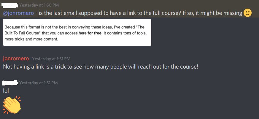 How many people will click to check out the website shouldn't matter when you are trying to validate a product.
 SaaS businesses (particularly ones for technical users) sometimes have to deal with a vocal outcry that their product “is just a wrapper around” something. The implication is that ‘a wrapper’ is inherently not valuable, and it’s impossible to build a great business around such a product. This logic is a product of lazy thinking and myopia; ‘wrappers’ can be insanely valuable.
 A hands-on guide for remote founders choosing where to incorporate. Real lessons, legal tips, and why Delaware keeps coming out on top.
 Short interview with Sergey Prilutskiy, developer, researcher, security specialist, co-founder of MixBytes company, and Hackernoon author.
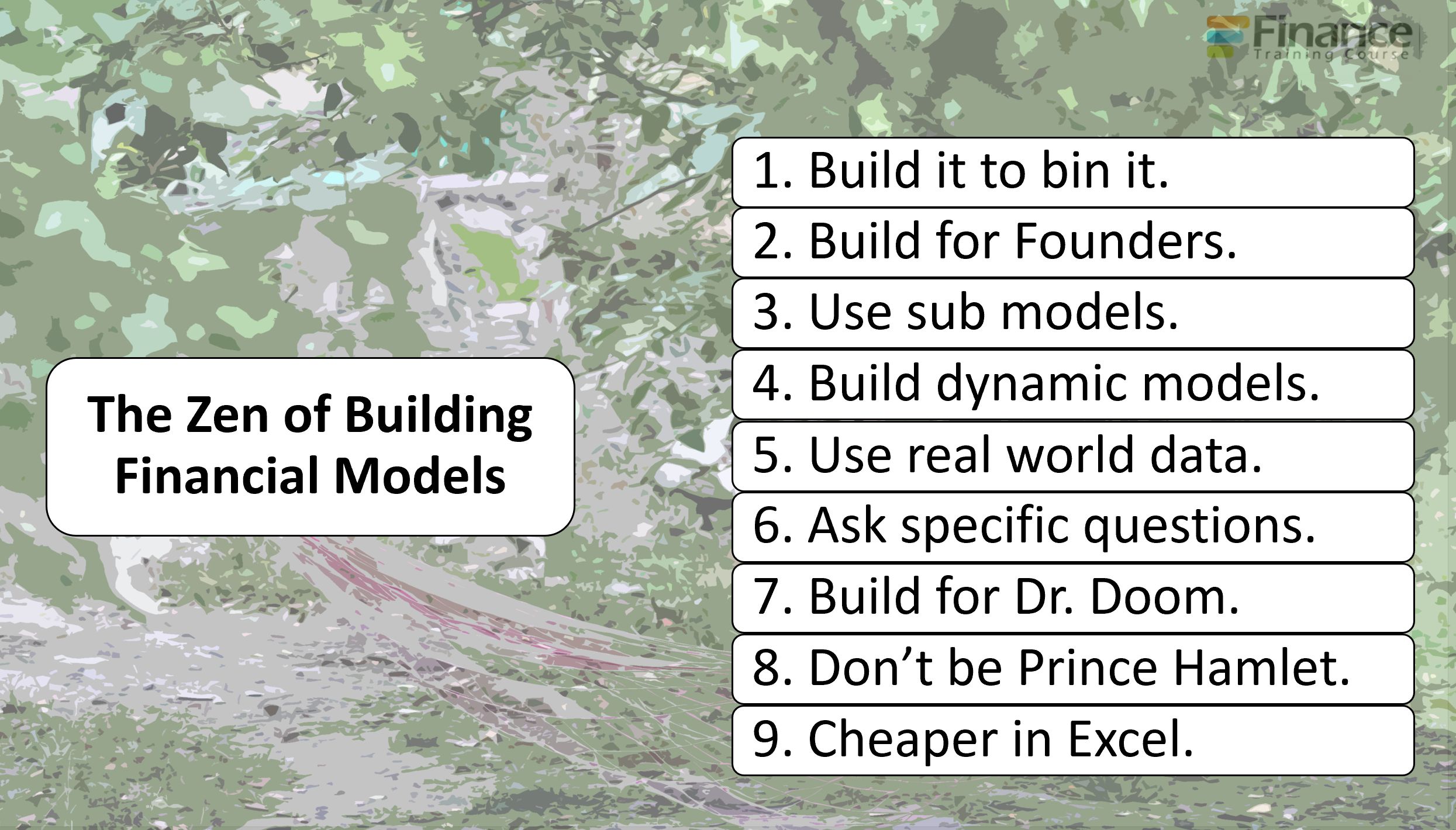 9 tips to improve your financial modeling game as a founder.
 Amy Tom chats with David Smooke (co-founder and CEO of HackerNoon) about his founder's journey with HackerNoon, and with Storm Farrell (Software Developer at Ha
 A “ready” UX designer is a rare encounter in the wild. Designers usually do know how to make things pretty – but when it comes to the product logic and interactions design, few feel at ease. The inevitable solution is to hire people with a relevant background and upgrade them to real UXers: host lectures, give homework, provide practice opportunities.
 Most founders skip a founder agreement because they trust each other. But when pressure hits - that missing structure becomes the root of chaos.
 Gennaro Cuofano (Italy) writes about digital business models, platforms, blockchain business models, and new ways of doing business, all the while managing the growth of a high-tech startup and a small sales team. In this interview: Decentralization, Scaling, and Building Your Own Platform.
 Do you need an advisor to help you through challenges? It’s another expense, not an immediate contribution to the top line. What to do?

 The restroom story
 It was in early 2025 that I initiated my own blog, OpenExploit.in, with one simple aim: to make cybersecurity easy to learn and available to all.
 Hey Hackernoon family! I havent contributed an article in a long time but I wanted to share how we grew our newsletter, Product Byte, to 497 subscribers and $150/mrr (6 paid members) before we even launched.
 In this episode of "Flying into the Future: How Tech is Shaping the Airlines Business," Omri Hurwitz welcomes esteemed guest Nathaniel Felsher.
 In this interview with Olayimika Oyebanji, Cam discussed EmpyrX and the importance of AI.
 If investors only know how to spot short-term, moonshot yields, is it possible that the overwhelming majority of successful startups get overlooked?
 Today, I want to talk to you about the life of information and how that fundamentally impacts remote working.
 If the game is unbeatable, frustration takes over and the game is tossed aside.
 It is 1943 and you are Head of the United States Eighth Air Force. Your mission is to destroy Germany's ability to wage war and free up the skies for the Allied Forces. The problem is that your Bombers are being zapped out of the sky like mosquitos drawn into the fire in a summery night.
 I am scared that more and more people are captivated by networked systems (and their tricks) that push them to move faster but not to become better thinkers.
 Startups love to talk about disruption, but when it comes to funding, the system still favors the familiar.
 10/15/2024: Top 5 stories on the HackerNoon homepage!
 Silverbird Founder Max Faldin about Building a Remote-First Startup
 Growing up and entering adulthood post-college, I always knew that I wanted to be in a position to help the Black community succeed and break barriers.
 A brief look at Twitch's humble beginnings, as well as pivotal decisions that turned their fortunes around.
 Learn how to strategically align investor relations with product growth for sustainable business success and revenue optimization.
 Hey HackerNoon Readers! I’m Nicolas and I’m the founder of Fortuitapps.
 Hayden Adams on Uniswap.
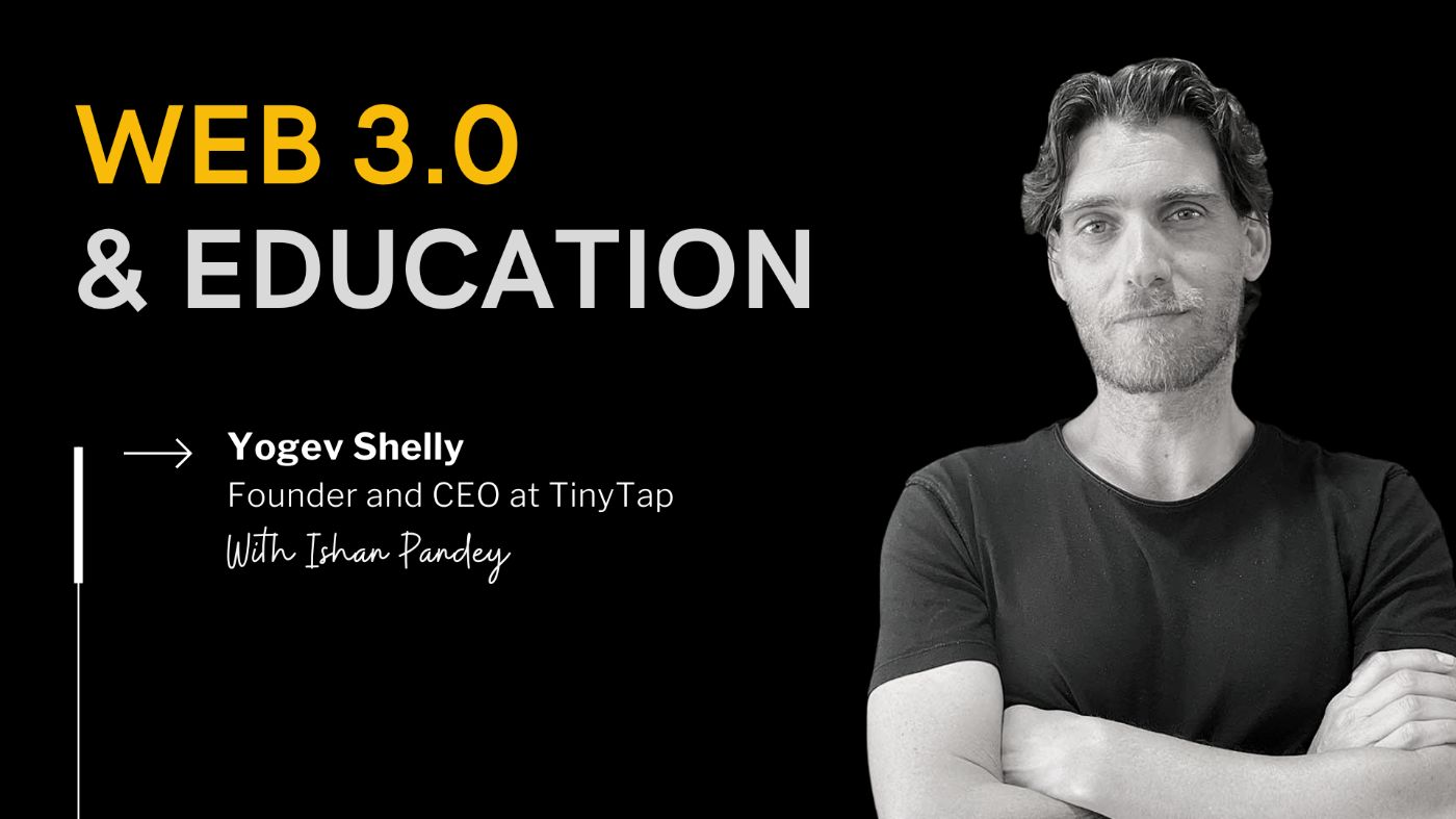 Yogev Shelly is the founder and CEO of TinyTap. TinyTap is the world’s largest library of educational games for young learners.
 Discover the journey of launching CoLaunchly, its challenges, and insights on startup life, burnout, and growth
 I’m normally a pretty big thinker. I like to analyze decisions and thoughts all the way out in the future and plan for all of the various contingencies. What happens if x goes wrong and then I’m in situation y? How will that affect a, b, and c? And I continue down the rabbit hole until I can’t see the light anymore.
 It pays to be neurodiverse - Ben Appleby escaped school and followed his instincts - now he is a co founder of an exciting web3 sporting platform launching soon
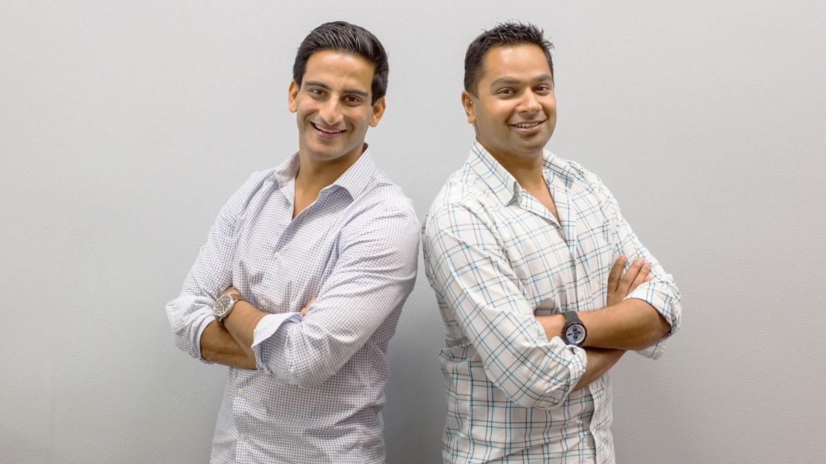 Unshackled Ventures founding partner Nitin Pachisia explains three ways he built a strong network during his fundraising journey.
 In mid-May, we were just closing our seed round after an 8-week-long fundraising process. Two weeks later, we started to have concerns over our product and vision. After a full month of interviews and explorations, we understood we needed to hard pivot. This article is about how we came to understand the shortcomings of our vision, and why we eventually decided to pivot. We talk about how we handled it with all the stakeholders (investors and team) in this article.
 Food trucks have been around for quite some time now, an idea sprung forth from an older necessity-driven idea, the chuckwagon. It is a simple proposition, really: instead of the public going to a restaurant or diner to eat, the food comes to them. One could consider it the older cousin of straight-to-your-door food delivery.
 I'm a mindset geek, It all comes down to that in the end, whether it's failures or wins. In my constant chase for Mindset hacks, tips and stories I had the opportunity to talk to the Digital Entrepreneur Marco Calamassi,
whose team develops social media brands and products for some of the biggest influencers. In this interview, I had a chance to ask a few questions regarding his journey, the struggles, the successes and the mindset needed. Here's what he had to say.
I'm a mindset geek, It all comes down to that in the end, whether it's failures or wins. In my constant chase for Mindset hacks, tips and stories I had the opportunity to talk to the Digital Entrepreneur Marco Calamassi,
whose team develops social media brands and products for some of the biggest influencers. In this interview, I had a chance to ask a few questions regarding his journey, the struggles, the successes and the mindset needed. Here's what he had to say.

 I share how taking full responsibility for risks (without hiding my fear) has shaped my leadership, empowered my team, and strengthened our company culture.
 Discover how well-meaning startup advice can backfire and learn practical strategies to avoid common pitfalls that slow your growth.
 Marzee Labs has launched its Manifesto on its website two years ago. The decision of writing it and the whole process we went through to get there was pretty cool and we wanted to tell you all about it. It made sense to be a team effort, so we brainstormed our way through it on a sunny and hot summer Saturday in Setúbal, Portugal, home of our designers.

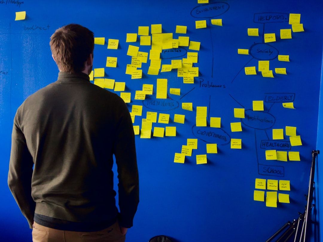 If you think you’ve prepared a brilliant deck full of numbers and charts, pause for a moment and make sure someone outside your project can understand it.
 Peace speaks with Erika Brodnock, Founder of Kami app.
 Bernard Moon is Venture Capitalist, Co-Founder of SparkLabs group and 3x Noonies nominee.
 Matt Huang assures people that Paradigm is committed to crypto.
 The difference between AI success and AI theater often comes down to this: did you start with a workflow, or did you start with a vision statement?
 I will give you three guesses as to why we chose to call the fund "Bostoncoin".
 Justin Caldbeck of Binary Capital explains similarities between basketball game and a venture capital firm.
 Hackernoon contributor Brian Wallace interviews Nachum Kligman, co-founder & CEO of Book Like a Boss.
Again, Take These Lessons With You](https://hackernoon.com/when-we-can-pitch-startups-at-events-again-take-these-lessons-with-you-in2jc3yio)
 Here I am, a twenty-year-old astrophysics student designing satellites to place in orbit around Mars and a self-starter entrepreneur longing to show my baby — nect MODEM — to the earth. I've had a few bumps on the road. Thankfully, I learned a few valuable lessons, and the experience of attending five conferences with my startup as my product made me reflect on a lot I'd like to share with other aspiring startup owners.
 He breaks down how one of his customers tapped into COLD leads (we’re talking 2-3 years old leads), and generated $16,000 dollars worth of brand-new business.
 As someone who went through the co-founder dating process (and emerged with a fantastic partner), I thought I’d share a few “real dating world" tips.
 Startup interview with Göran Almgren, co-founder, Enigio.
 Few years ago, I consulted for a small Rx delivery startup in HongKong where I focused on strategy, go-to-market and built out their product direction from the
 Building 100+ Year Brands: We nurture long-lasting, impactful brands, guiding e-commerce founders to monumental growth and cultural influence.
 Our investor update guide includes a template and best practices, including why you should send updates before you even have investors.
 Your first finance hire will shape how your company understands itself. Below $1M ARR, structure is more important than headcount. From $1M to $10M, your financ
 The survey covered 13 questions, meant to elicit both open-ended qualitative responses, as well as structured rankings of common challenges
 Let’s admit it.
Typical software is old-school in the tech industry now.
Companies find subscription-based services more comfy these days.
Are you still toying
Let’s admit it.
Typical software is old-school in the tech industry now.
Companies find subscription-based services more comfy these days.
Are you still toying
 Why great presentations still fail to convince decision-makers. Learn how to turn decks from information overload into clear paths that drive real decisions.
 Discover how to scale a VR startup globally, cut hardware costs, and build sustainable models for small businesses.
 The domain of enterprise software is littered with acronyms that may be intimidating even to seasoned managers. Things get even murkier for those seeking to develop their own mobile enterprise app and encountering design-specific terms. The fact that some of them are often used interchangeably also doesn’t help. So the best place to start figuring out these terms is to understand their similarities and differences and identify the areas where they overlap.
 Never Trusting Anybody, and the Impact it Had on Me
 As a company founder, I’ve received my fair share of advice over the years. Some of it has been instrumental in helping me build my startup. Others, well, not so much.
 Was there a big risk trying a startup? Did you have any sort of security net to catch you if you fall? and other questions get answered
 Leia Ruseva from India has been nominated for a 2020 #Noonie in the Future Heroes and Technology categories.
 I am pretty sure you’ve heard the saying that you are the average of the 5 people surrounding you, right? I have something to tell you that it is terrifying: It is bullshit, because it's worse.
 You know that feeling when you work really hard on something for really long and it feels like nobody really notices?
 The tech workforce in the US is not growing at an optimal pace. The number of schools offering computer science is not enough which is impacting the access of computer science to young women and students from marginalized communities.
 Founders often publish commitments before the system is ready. A systems-level look at how language becomes an interface, and creates irreversible coupling.
 Most founders obsess over their failures, completely ignoring times of clarity and small wins.
Visit the /Learn Repo to find the most read blog posts about any technology.