2025-01-16 08:00:00
As we’re still in the early days of building applications with foundation models, it’s normal to make mistakes. This is a quick note with examples of some of the most common pitfalls that I’ve seen, both from public case studies and from my personal experience.
Because these pitfalls are common, if you’ve worked on any AI product, you’ve probably seen them before.
Every time there’s a new technology, I can hear the collective sigh of senior engineers everywhere: “Not everything is a nail.” Generative AI isn’t an exception — its seemingly limitless capabilities only exacerbate the tendency to use generative AI for everything.
A team pitched me the idea of using generative AI to optimize energy consumption. They fed a household’s list of energy-intensive activities and hourly electricity prices into an LLM, then asked it to create a schedule to minimize energy costs. Their experiments showed that this could help reduce a household’s electricity bill by 30%. Free money. Why wouldn’t anyone want to use their app?
I asked: “How does it compare to simply scheduling the most energy-intensive activities when electricity is cheapest? Say, doing your laundry and charging your car after 10pm?”
They said they would try it later and let me know. They never followed up, but they abandoned this app soon after. I suspect that this greedy scheduling can be quite effective. Even if it’s not, there are other much cheaper and more reliable optimization solutions than generative AI, like linear programming.
I’ve seen this scenario over and over again. A big company wants to use generative AI to detect anomalies in network traffic. Another wants to predict upcoming customer call volume. A hospital wants to detect whether a patient is malnourished (really not recommended).
It can often be beneficial to explore a new approach to get a sense of what’s possible, as long as you’re aware that your goal isn’t to solve a problem but to test a solution. “We solve the problem” and “We use generative AI” are two very different headlines, and unfortunately, so many people would rather have the latter.
At the other end of the spectrum, many teams dismiss gen AI as a valid solution for their problems because they tried it out and their users hated it. However, other teams successfully used gen AI for similar use cases. I could only look into two of these teams. In both cases, the issue wasn’t with AI, but with product.
Many people have told me that the technical aspects of their AI applications are straightforward. The hard part is user experience (UX). What should the product interface look like? How to seamlessly integrate the product into the user workflow? How to incorporate human-in-the-loop?
UX has always been challenging, but it’s even more so with generative AI. While we know that generative AI is changing how we read, write, learn, teach, work, entertain, etc., we don’t quite know how yet. What will the future of reading/learning/working be like?
Here are some simple examples to show how what users want can be counter-intuitive and need rigorous user study.
My friend works on an application that summarizes meeting transcripts. Initially, her team focused on getting the right summary length. Would users prefer 3-sentence summaries or 5-sentence summaries?
However, it turned out that their users didn’t care about the actual summary. They only wanted action items specific to them from each meeting.
When LinkedIn developed a chatbot for skill fit assessment, they discovered that users didn’t want correct responses. Users wanted helpful responses.
For example, if a user asks a bot whether they’re a fit for a job and the bot responds with: “You’re a terrible fit,” this response might be correct but not very helpful to the user. Users want tips on what the gaps are and what they can do to close the gaps.
Intuit built a chatbot to help users answer tax questions. Initially, they got lukewarm feedback — users didn’t find the bot useful. After investigation, they found out that users actually hated typing. Facing a blank chatbot, users didn’t know what the bot could do and what to type.
So, for each interaction, Intuit added a few suggested questions for users to click on. This reduced the friction for users to use the bot and gradually built users’ trust. The feedback from users then became much more positive.
(Shared by Nhung Ho, VP of AI at Intuit, during our panel at Grace Hopper.)
Because everyone uses the same models nowadays, the AI components of AI products are similar, and the differentiation is product.
Examples of this pitfall:
Given so many shiny new technologies, it’s tempting to jump straight into using them. However, incorporating external tools too early can cause 2 problems:
Tool developers can make mistakes. For example, I often find typos in default prompts when reviewing a framework’s codebase. If the framework you use updates its prompt without telling you, your application’s behaviors might change and you might not know why.
Eventually, abstractions are good. But abstractions need to incorporate best practices and be tested overtime. As we’re still in the early days of AI engineering, best practices are still evolving, we should be more vigilant when adopting any abstraction.
It took LinkedIn 1 month to achieve 80% of the experience they wanted, and an additional 4 months to surpass 95%. The initial success made them grossly underestimate how challenging it is to improve the product, especially around hallucinations. They found it discouraging how difficult it was to achieve each subsequent 1% gain.
"talk like a luxury brand concierge") in the system prompt to be perfectly obeyedThanks Jason Tjahjono for sharing this.
This is perhaps one of the first painful lessons anyone who has built an AI product quickly learns. It’s easy to build a demo, but hard to build a product. Other than the issues of hallucinations, latency, latency/accuracy tradeoff, tool use, prompting, testing, … as mentioned, teams also run into issues, such as:
When planning a product’s milestones and resources, make sure to take into account these potential roadblocks. A friend calls this “being cautiously optimistic”. However, remember that many cool demos don’t lead to wonderful products.
To automatically evaluate AI applications, many teams opt for the AI-as-a-judge (also called LLM-as-a-judge) approach — using AI models to evaluate AI outputs. A common pitfall is forgoing human evaluation to rely entirely on AI judges.
While AI judges can be very useful, they aren’t deterministic. The quality of a judge depends on the underlying judge’s model, the judge’s prompt, and the use case. If the AI judge isn’t developed properly, it can give misleading evaluations about your application’s performance. AI judges must be evaluated and iterated over time, just like all other AI applications.

The teams with the best products I’ve seen all have human evaluation to supplement their automated evaluation. Every day, they have human experts evaluate a subset of their application’s outputs, which can be anywhere from 30 - 1000 examples.
Daily manual evaluation serves 3 purposes:
The reliability of human evaluation also depends on well-crafted annotation guidelines. These annotation guidelines can help improve the model’s instructions (if a human has a hard time following the instructions, the model will, too). It can also be reused to create finetuning data later if you choose to finetune.
In every project I’ve worked on, staring at data for just 15 minutes usually gives me some insight that could save me hours of headaches. Greg Brockman tweeted: “Manual inspection of data has probably the highest value-to-prestige ratio of any activity in machine learning.”
This is a mistake I saw in the early days when enterprises were in a frenzy to adopt generative AI. Unable to come up with a strategy for what use cases to focus on, many tech executives crowdsourced ideas from the whole company. “We hire smart people. Let them tell us what to do.” They then try to implement these ideas one by one.
And that’s how we ended up with a million text-to-SQL models, a million Slack bots, and a billion code plugins.
While it’s indeed a good idea to listen to the smart people that you hire, individuals might be biased toward the problems that immediately affect their day-to-day work instead of problems that might bring the highest returns on investment. Without an overall strategy that considers the big picture, it’s easy to get sidetracked into a series of small, low-impact applications and come to the wrong conclusion that gen AI has no ROI.
In short, here are the common AI engineering pitfalls:
Use generative AI when you don’t need generative AI
Gen AI isn’t a one-size-fits-all solution to all problems. Many problems don’t even need AI.
Confuse ‘bad product’ with ‘bad AI’
For many AI product, AI is the easy part, product is the hard part.
Start too complex
While fancy new frameworks and finetuning can be useful for many projects, they shouldn’t be your first course of action.
Over-index on early success
Initial success can be misleading. Going from demo-ready to production-ready can take much longer than getting to the first demo.
Forgo human evaluation
AI judges should be validated and correlated with systematic human evaluation.
Crowdsource use cases
Have a big-picture strategy to maximize return on investment.
2025-01-07 08:00:00
Intelligent agents are considered by many to be the ultimate goal of AI. The classic book by Stuart Russell and Peter Norvig, Artificial Intelligence: A Modern Approach (Prentice Hall, 1995), defines the field of AI research as “the study and design of rational agents.”
The unprecedented capabilities of foundation models have opened the door to agentic applications that were previously unimaginable. These new capabilities make it finally possible to develop autonomous, intelligent agents to act as our assistants, coworkers, and coaches. They can help us create a website, gather data, plan a trip, do market research, manage a customer account, automate data entry, prepare us for interviews, interview our candidates, negotiate a deal, etc. The possibilities seem endless, and the potential economic value of these agents is enormous.
This section will start with an overview of agents and then continue with two aspects that determine the capabilities of an agent: tools and planning. Agents, with their new modes of operations, have new modes of failure. This section will end with a discussion on how to evaluate agents to catch these failures.
This post is adapted from the Agents section of AI Engineering (2025) with minor edits to make it a standalone post.
Notes:
The term agent has been used in many different engineering contexts, including but not limited to a software agent, intelligent agent, user agent, conversational agent, and reinforcement learning agent. So, what exactly is an agent?
An agent is anything that can perceive its environment and act upon that environment. Artificial Intelligence: A Modern Approach (1995) defines an agent as anything that can be viewed as perceiving its environment through sensors and acting upon that environment through actuators.
This means that an agent is characterized by the environment it operates in and the set of actions it can perform.
The environment an agent can operate in is defined by its use case. If an agent is developed to play a game (e.g., Minecraft, Go, Dota), that game is its environment. If you want an agent to scrape documents from the internet, the environment is the internet. A self-driving car agent’s environment is the road system and its adjacent areas.
The set of actions an AI agent can perform is augmented by the tools it has access to. Many generative AI-powered applications you interact with daily are agents with access to tools, albeit simple ones. ChatGPT is an agent. It can search the web, execute Python code, and generate images. RAG systems are agents—text retrievers, image retrievers, and SQL executors are their tools.
There’s a strong dependency between an agent’s environment and its set of tools. The environment determines what tools an agent can potentially use. For example, if the environment is a chess game, the only possible actions for an agent are the valid chess moves. However, an agent’s tool inventory restricts the environment it can operate in. For example, if a robot’s only action is swimming, it’ll be confined to a water environment.
Figure 6-8 shows a visualization of SWE-agent (Yang et al., 2024), an agent built on top of GPT-4. Its environment is the computer with the terminal and the file system. Its set of actions include navigate repo, search files, view files, and edit lines.

An AI agent is meant to accomplish tasks typically provided by the users. In an AI agent, AI is the brain that processes the task, plans a sequence of actions to achieve this task, and determines whether the task has been accomplished.
Let’s return to the RAG system with tabular data in the Kitty Vogue example above. This is a simple agent with three actions:
Given the query "Project the sales revenue for Fruity Fedora over the next three months", the agent might perform the following sequence of actions:
Compared to non-agent use cases, agents typically require more powerful models for two reasons:
A task that requires many steps can take time and money to run. A common complaint is that agents are only good for burning through your API credits. However, if agents can be autonomous, they can save human time, making their costs worthwhile.
Given an environment, the success of an agent in an environment depends on the tool it has access to and the strength of its AI planner. Let’s start by looking into different kinds of tools a model can use. We’ll analyze AI’s capability for planning next.
A system doesn’t need access to external tools to be an agent. However, without external tools, the agent’s capabilities would be limited. By itself, a model can typically perform one action—an LLM can generate text and an image generator can generate images. External tools make an agent vastly more capable.
Tools help an agent to both perceive the environment and act upon it. Actions that allow an agent to perceive the environment are read-only actions, whereas actions that allow an agent to act upon the environment are write actions.
The set of tools an agent has access to is its tool inventory. Since an agent’s tool inventory determines what an agent can do, it’s important to think through what and how many tools to give an agent. More tools give an agent more capabilities. However, the more tools there are, the more challenging it is to understand and utilize them well. Experimentation is necessary to find the right set of tools, as discussed later in the “Tool selection” section.
Depending on the agent’s environment, there are many possible tools. Here are three categories of tools that you might want to consider: knowledge augmentation (i.e., context construction), capability extension, and tools that let your agent act upon its environment.
I hope that this book, so far, has convinced you of the importance of having the relevant context for a model’s response quality. An important category of tools includes those that help augment the knowledge of your agent. Some of them have already been discussed: text retriever, image retriever, and SQL executor. Other potential tools include internal people search, an inventory API that returns the status of different products, Slack retrieval, an email reader, etc.
Many such tools augment a model with your organization’s private processes and information. However, tools can also give models access to public information, especially from the internet.
Web browsing was among the earliest and most anticipated capabilities to be incorporated into ChatGPT. Web browsing prevents a model from going stale. A model goes stale when the data it was trained on becomes outdated. If the model’s training data was cut off last week, it won’t be able to answer questions that require information from this week unless this information is provided in the context. Without web browsing, a model won’t be able to tell you about the weather, news, upcoming events, stock prices, flight status, etc.
I use web browsing as an umbrella term to cover all tools that access the internet, including web browsers and APIs such as search APIs, news APIs, GitHub APIs, or social media APIs.
While web browsing allows your agent to reference up-to-date information to generate better responses and reduce hallucinations, it can also open up your agent to the cesspools of the internet. Select your Internet APIs with care.
You might also consider tools that address the inherent limitations of AI models. They are easy ways to give your model a performance boost. For example, AI models are notorious for being bad at math. If you ask a model what is 199,999 divided by 292, the model will likely fail. However, this calculation would be trivial if the model had access to a calculator. Instead of trying to train the model to be good at arithmetic, it’s a lot more resource-efficient to just give the model access to a tool.
Other simple tools that can significantly boost a model’s capability include a calendar, timezone converter, unit converter (e.g., from lbs to kg), and translator that can translate to and from the languages that the model isn’t good at.
More complex but powerful tools are code interpreters. Instead of training a model to understand code, you can give it access to a code interpreter to execute a piece of code, return the results, or analyze the code’s failures. This capability lets your agents act as coding assistants, data analysts, and even research assistants that can write code to run experiments and report results. However, automated code execution comes with the risk of code injection attacks, as discussed in Chapter 5 in the section “Defensive Prompt Engineering“. Proper security measurements are crucial to keep you and your users safe.
Tools can turn a text-only or image-only model into a multimodal model. For example, a model that can generate only texts can leverage a text-to-image model as a tool, allowing it to generate both texts and images. Given a text request, the agent’s AI planner decides whether to invoke text generation, image generation, or both. This is how ChatGPT can generate both text and images—it uses DALL-E as its image generator.
Agents can also use a code interpreter to generate charts and graphs, a LaTex compiler to render math equations, or a browser to render web pages from HTML code.
Similarly, a model that can process only text inputs can use an image captioning tool to process images and a transcription tool to process audio. It can use an OCR (optical character recognition) tool to read PDFs.
Tool use can significantly boost a model’s performance compared to just prompting or even finetuning. Chameleon (Lu et al., 2023) shows that a GPT-4-powered agent, augmented with a set of 13 tools, can outperform GPT-4 alone on several benchmarks. Examples of tools this agent used are knowledge retrieval, a query generator, an image captioner, a text detector, and Bing search.
On ScienceQA, a science question answering benchmark, Chameleon improves the best published few-shot result by 11.37%. On TabMWP (Tabular Math Word Problems) (Lu et al., 2022), a benchmark involving tabular math questions, Chameleon improves the accuracy by 17%.
So far, we’ve discussed read-only actions that allow a model to read from its data sources. But tools can also perform write actions, making changes to the data sources. An SQL executor can retrieve a data table (read) and change or delete the table (write). An email API can read an email but can also respond to it. A banking API can retrieve your current balance, but can also initiate a bank transfer.
Write actions enable a system to do more. They can enable you to automate the whole customer outreach workflow: researching potential customers, finding their contacts, drafting emails, sending first emails, reading responses, following up, extracting orders, updating your databases with new orders, etc.
However, the prospect of giving AI the ability to automatically alter our lives is frightening. Just as you shouldn’t give an intern the authority to delete your production database, you shouldn’t allow an unreliable AI to initiate bank transfers. Trust in the system’s capabilities and its security measures is crucial. You need to ensure that the system is protected from bad actors who might try to manipulate it into performing harmful actions.
Sidebar: Agents and security
Whenever I talk about autonomous AI agents to a group of people, there is often someone who brings up self-driving cars. “What if someone hacks into the car to kidnap you?” While the self-driving car example seems visceral because of its physicality, an AI system can cause harm without a presence in the physical world. It can manipulate the stock market, steal copyrights, violate privacy, reinforce biases, spread misinformation and propaganda, and more, as discussed in the section “Defensive Prompt Engineering” in Chapter 5.
These are all valid concerns, and any organization that wants to leverage AI needs to take safety and security seriously. However, this doesn’t mean that AI systems should never be given the ability to act in the real world. If we can trust a machine to take us into space, I hope that one day, security measures will be sufficient for us to trust autonomous AI systems. Besides, humans can fail, too. Personally, I would trust a self-driving car more than the average stranger to give me a lift.
Just as the right tools can help humans be vastly more productive—can you imagine doing business without Excel or building a skyscraper without cranes?—tools enable models to accomplish many more tasks. Many model providers already support tool use with their models, a feature often called function calling. Going forward, I would expect function calling with a wide set of tools to be common with most models.
At the heart of a foundation model agent is the model responsible for solving user-provided tasks. A task is defined by its goal and constraints. For example, one task is to schedule a two-week trip from San Francisco to India with a budget of $5,000. The goal is the two-week trip. The constraint is the budget.
Complex tasks require planning. The output of the planning process is a plan, which is a roadmap outlining the steps needed to accomplish a task. Effective planning typically requires the model to understand the task, consider different options to achieve this task, and choose the most promising one.
If you’ve ever been in any planning meeting, you know that planning is hard. As an important computational problem, planning is well studied and would require several volumes to cover. I’ll only be able to cover the surface here.
Given a task, there are many possible ways to solve it, but not all of them will lead to a successful outcome. Among the correct solutions, some are more efficient than others. Consider the query, "How many companies without revenue have raised at least $1 billion?", and the two example solutions:
The second option is more efficient. There are vastly more companies without revenue than companies that have raised $1 billion. Given only these two options, an intelligent agent should choose option 2.
You can couple planning with execution in the same prompt. For example, you give the model a prompt, ask it to think step by step (such as with a chain-of-thought prompt), and then execute those steps all in one prompt. But what if the model comes up with a 1,000-step plan that doesn’t even accomplish the goal? Without oversight, an agent can run those steps for hours, wasting time and money on API calls, before you realize that it’s not going anywhere.
To avoid fruitless execution, planning should be decoupled from execution. You ask the agent to first generate a plan, and only after this plan is validated is it executed. The plan can be validated using heuristics. For example, one simple heuristic is to eliminate plans with invalid actions. If the generated plan requires a Google search and the agent doesn’t have access to Google Search, this plan is invalid. Another simple heuristic might be eliminating all plans with more than X steps.
A plan can also be validated using AI judges. You can ask a model to evaluate whether the plan seems reasonable or how to improve it.
If the generated plan is evaluated to be bad, you can ask the planner to generate another plan. If the generated plan is good, execute it.
If the plan consists of external tools, function calling will be invoked. Outputs from executing this plan will then again need to be evaluated. Note that the generated plan doesn’t have to be an end-to-end plan for the whole task. It can be a small plan for a subtask. The whole process looks like Figure 6-9.
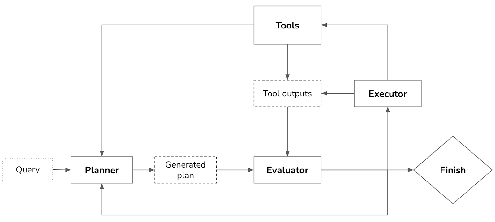
Your system now has three components: one to generate plans, one to validate plans, and another to execute plans. If you consider each component an agent, this can be considered a multi-agent system. Because most agentic workflows are sufficiently complex to involve multiple components, most agents are multi-agent.
To speed up the process, instead of generating plans sequentially, you can generate several plans in parallel and ask the evaluator to pick the most promising one. This is another latency–cost tradeoff, as generating multiple plans simultaneously will incur extra costs.
Planning requires understanding the intention behind a task: what’s the user trying to do with this query? An intent classifier is often used to help agents plan. As shown in Chapter 5 in the section “Break complex tasks into simpler subtasks“, intent classification can be done using another prompt or a classification model trained for this task. The intent classification mechanism can be considered another agent in your multi-agent system.
Knowing the intent can help the agent pick the right tools. For example, for customer support, if the query is about billing, the agent might need access to a tool to retrieve a user’s recent payments. But if the query is about how to reset a password, the agent might need to access documentation retrieval.
Tip:
Some queries might be out of the scope of the agent. The intent classifier should be able to classify requests as
IRRELEVANTso that the agent can politely reject those instead of wasting FLOPs coming up with impossible solutions.
So far, we’ve assumed that the agent automates all three stages: generating plans, validating plans, and executing plans. In reality, humans can be involved at any stage to aid with the process and mitigate risks.
To summarize, solving a task typically involves the following processes. Note that reflection isn’t mandatory for an agent, but it’ll significantly boost the agent’s performance.
You’ve already seen some techniques for plan generation and reflection in this book. When you ask a model to “think step by step”, you’re asking it to decompose a task. When you ask a model to “verify if your answer is correct”, you’re asking it to reflect.
An open question is how well foundation models can plan. Many researchers believe that foundation models, at least those built on top of autoregressive language models, cannot. Meta’s Chief AI Scientist Yann LeCun states unequivocably that autoregressive LLMs can’t plan (2023).
Auto-Regressive LLMs can't plan
— Yann LeCun (@ylecun) September 13, 2023
(and can't really reason).
"While our own limited experiments didn't show any significant improvement [in planning abilities] through fine tuning, it is possible that with even more fine tuning data and effort, the empirical performance may well… https://t.co/rHA5QHi90C
While there is a lot of anecdotal evidence that LLMs are poor planners, it’s unclear whether it’s because we don’t know how to use LLMs the right way or because LLMs, fundamentally, can’t plan.
Planning, at its core, is a search problem. You search among different paths towards the goal, predict the outcome (reward) of each path, and pick the path with the most promising outcome. Often, you might determine that no path exists that can take you to the goal.
Search often requires backtracking. For example, imagine you’re at a step where there are two possible actions: A and B. After taking action A, you enter a state that’s not promising, so you need to backtrack to the previous state to take action B.
Some people argue that an autoregressive model can only generate forward actions. It can’t backtrack to generate alternate actions. Because of this, they conclude that autoregressive models can’t plan. However, this isn’t necessarily true. After executing a path with action A, if the model determines that this path doesn’t make sense, it can revise the path using action B instead, effectively backtracking. The model can also always start over and choose another path.
It’s also possible that LLMs are poor planners because they aren’t given the toolings needed to plan. To plan, it’s necessary to know not only the available actions but also the potential outcome of each action. As a simple example, let’s say you want to walk up a mountain. Your potential actions are turn right, turn left, turn around, or go straight ahead. However, if turning right will cause you to fall off the cliff, you might not consider this action. In technical terms, an action takes you from one state to another, and it’s necessary to know the outcome state to determine whether to take an action.
This means that prompting a model to generate only a sequence of actions like what the popular chain-of-thought prompting technique does isn’t sufficient. The paper “Reasoning with Language Model is Planning with World Model” (Hao et al., 2023) argues that an LLM, by containing so much information about the world, is capable of predicting the outcome of each action. This LLM can incorporate this outcome prediction to generate coherent plans.
Even if AI can’t plan, it can still be a part of a planner. It might be possible to augment an LLM with a search tool and state tracking system to help it plan.
Sidebar: Foundation model (FM) versus reinforcement learning (RL) planners
The agent is a core concept in RL, which is defined in Wikipedia as a field “concerned with how an intelligent agent ought to take actions in a dynamic environment in order to maximize the cumulative reward.”
RL agents and FM agents are similar in many ways. They are both characterized by their environments and possible actions. The main difference is in how their planners work.
However, there’s nothing to prevent an FM agent from incorporating RL algorithms to improve its performance. I suspect that in the long run, FM agents and RL agents will merge.
The simplest way to turn a model into a plan generator is with prompt engineering. Imagine that you want to create an agent to help customers learn about products at Kitty Vogue. You give this agent access to three external tools: retrieve products by price, retrieve top products, and retrieve product information. Here’s an example of a prompt for plan generation. This prompt is for illustration purposes only. Production prompts are likely more complex.
SYSTEM PROMPT:
Propose a plan to solve the task. You have access to 5 actions:

* get_today_date()
* fetch_top_products(start_date, end_date, num_products)
* fetch_product_info(product_name)
* generate_query(task_history, tool_output)
* generate_response(query)

The plan must be a sequence of valid actions.

Examples
Task: "Tell me about Fruity Fedora"
Plan: [fetch_product_info, generate_query, generate_response]

Task: "What was the best selling product last week?"
Plan: [fetch_top_products, generate_query, generate_response]

Task: {USER INPUT}
Plan:
There are two things to note about this example:
generate_query function takes in the task’s current history and the most recent tool outputs to generate a query to be fed into the response generator. The tool output at each step is added to the task’s history.Given the user input “What’s the price of the best-selling product last week”, a generated plan might look like this:
get_time()fetch_top_products()fetch_product_info()generate_query()generate_response()You might wonder, “What about the parameters needed for each function?” The exact parameters are hard to predict in advance since they are often extracted from the previous tool outputs. If the first step, get_time(), outputs “2030-09-13”, the agent can reason that the parameters for the next step should be called with the following parameters:
fetch_top_products(
    start_date="2030-09-07",
    end_date="2030-09-13",
    num_products=1
)
Often, there’s insufficient information to determine the exact parameter values for a function. For example, if a user asks “What’s the average price of best-selling products?”, the answers to the following questions are unclear:
This means that models frequently have to make guesses, and guesses can be wrong.
Because both the action sequence and the associated parameters are generated by AI models, they can be hallucinated. Hallucinations can cause the model to call an invalid function or call a valid function but with wrong parameters. Techniques for improving a model’s performance in general can be used to improve a model’s planning capabilities.
Tips for making an agent better at planning.
- Write a better system prompt with more examples.
- Give better descriptions of the tools and their parameters so that the model understands them better.
- Rewrite the functions themselves to make them simpler, such as refactoring a complex function into two simpler functions.
- Use a stronger model. In general, stronger models are better at planning.
- Finetune a model for plan generation.
Many model providers offer tool use for their models, effectively turning their models into agents. A tool is a function. Invoking a tool is, therefore, often called function calling. Different model APIs work differently, but in general, function calling works as follows:
required: the model must use at least one tool.none: the model shouldn’t use any tool.auto: the model decides which tools to use.Function calling is illustrated in Figure 6-10. This is written in pseudocode to make it representative of multiple APIs. To use a specific API, please refer to its documentation.
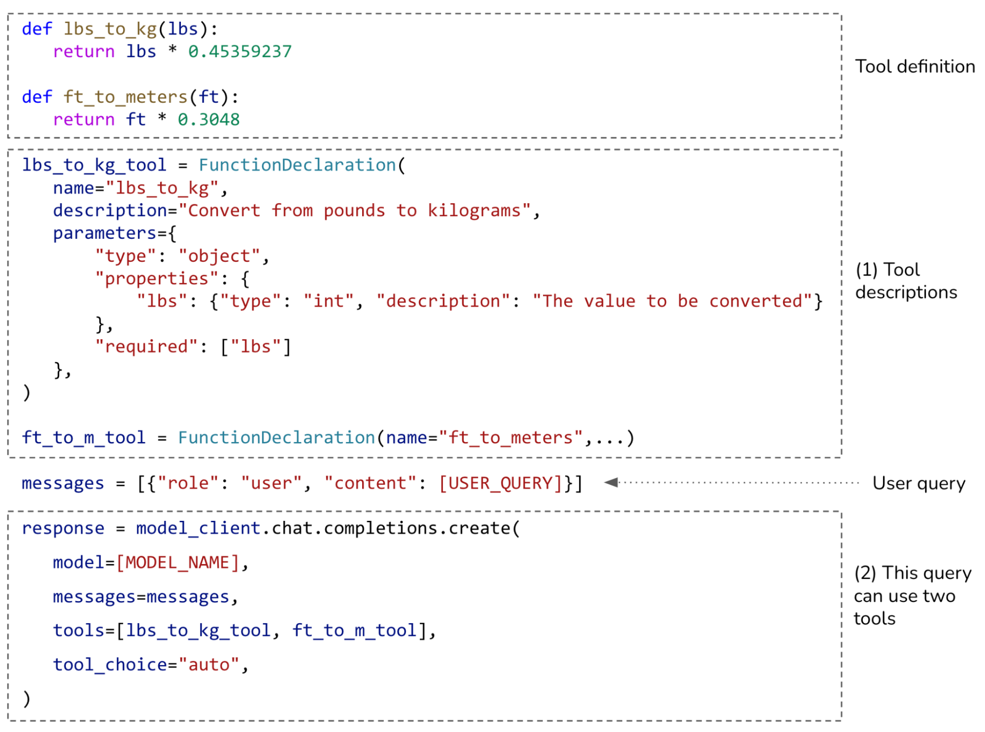
Given a query, an agent defined as in Figure 6-10 will automatically generate what tools to use and their parameters. Some function calling APIs will make sure that only valid functions are generated, though they won’t be able to guarantee the correct parameter values.
For example, given the user query “How many kilograms are 40 pounds?”, the agent might decide that it needs the tool lbs_to_kg_tool with one parameter value of 40. The agent’s response might look like this.
response = ModelResponse(
    finish_reason='tool_calls',
    message=chat.Message(
        content=None,
        role='assistant',
        tool_calls=[
            ToolCall(
                function=Function(
                    arguments='{"lbs":40}',
                    name='lbs_to_kg'),
                type='function')
        ])
)
From this response, you can evoke the function lbs_to_kg(lbs=40) and use its output to generate a response to the users.
Tip: When working with agents, always ask the system to report what parameter values it uses for each function call. Inspect these values to make sure they are correct.
A plan is a roadmap outlining the steps needed to accomplish a task. A roadmap can be of different levels of granularity. To plan for a year, a quarter-by-quarter plan is higher-level than a month-by-month plan, which is, in turn, higher-level than a week-to-week plan.
There’s a planning/execution tradeoff. A detailed plan is harder to generate, but easier to execute. A higher-level plan is easier to generate, but harder to execute. An approach to circumvent this tradeoff is to plan hierarchically. First, use a planner to generate a high-level plan, such as a quarter-to-quarter plan. Then, for each quarter, use the same or a different planner to generate a month-to-month plan.
So far, all examples of generated plans use the exact function names, which is very granular. A problem with this approach is that an agent’s tool inventory can change over time. For example, the function to get the current date get_time() can be renamed to get_current_time(). When a tool changes, you’ll need to update your prompt and all your examples. Using the exact function names also makes it harder to reuse a planner across different use cases with different tool APIs.
If you’ve previously finetuned a model to generate plans based on the old tool inventory, you’ll need to finetune the model again on the new tool inventory.
To avoid this problem, plans can also be generated using a more natural language, which is higher-level than domain-specific function names. For example, given the query “What’s the price of the best-selling product last week”, an agent can be instructed to output a plan that looks like this:
get current dateretrieve the best-selling product last weekretrieve product informationgenerate querygenerate responseUsing more natural language helps your plan generator become robust to changes in tool APIs. If your model was trained mostly on natural language, it’ll likely be better at understanding and generating plans in natural language and less likely to hallucinate.
The downside of this approach is that you need a translator to translate each natural language action into executable commands. Chameleon (Lu et al., 2023) calls this translator a program generator. However, translating is a much simpler task than planning and can be done by weaker models with a lower risk of hallucination.
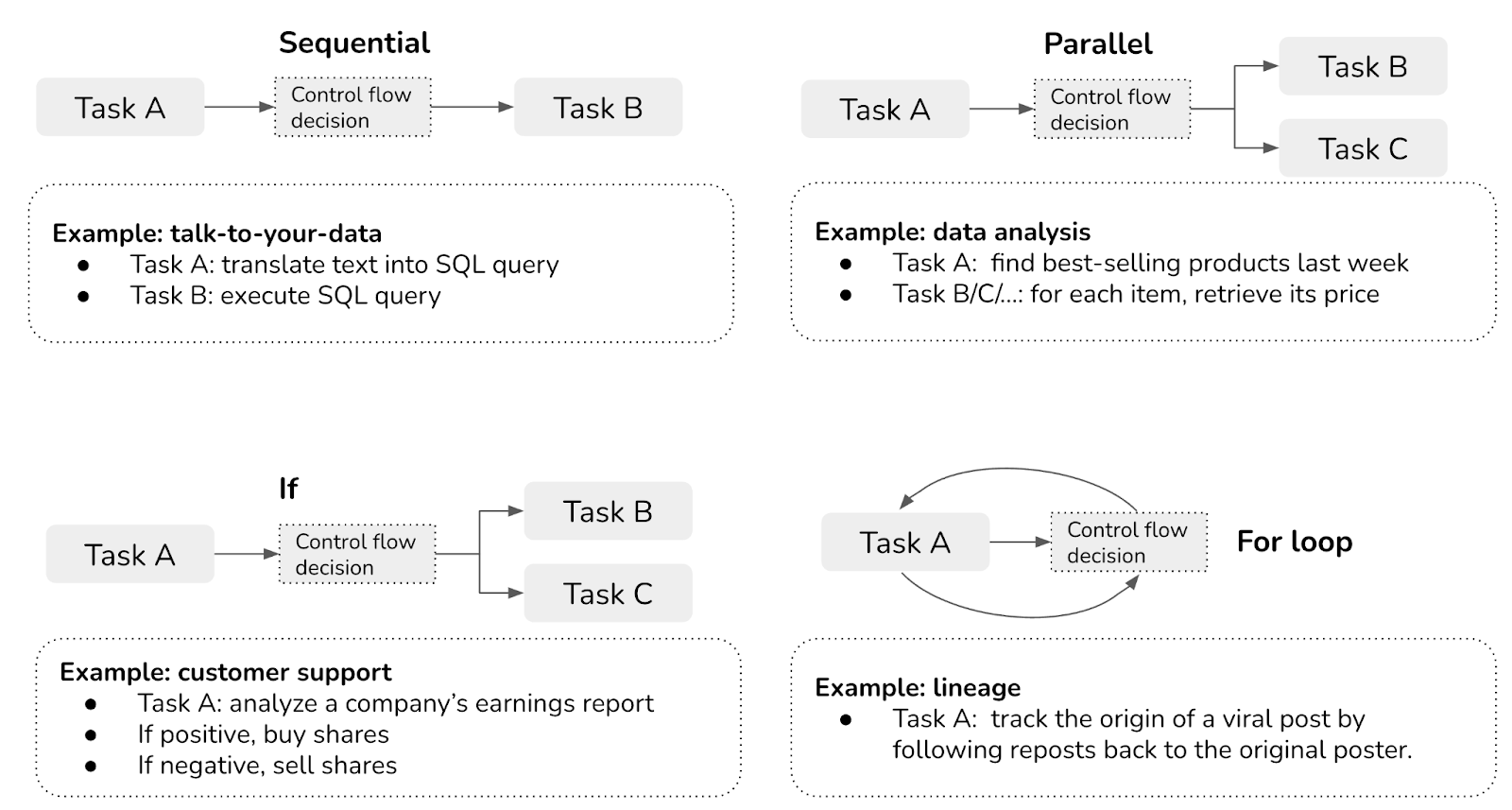
The plan examples so far have been sequential: the next action in the plan is always executed after the previous action is done. The order in which actions can be executed is called a control flow. The sequential form is just one type of control flow. Other types of control flows include the parallel, if statement, and for loop. The list below provides an overview of each control flow, including sequential for comparison:
Sequential
Executing task B after task A is complete, possibly because task B depends on task A. For example, the SQL query can only be executed after it’s been translated from the natural language input.
Parallel
Executing tasks A and B at the same time. For example, given the query “Find me best-selling products under $100”, an agent might first retrieve the top 100 best-selling products and, for each of these products, retrieve its price.
If statement
Executing task B or task C depending on the output from the previous step. For example, the agent first checks NVIDIA’s earnings report. Based on this report, it can then decide to sell or buy NVIDIA stocks. Anthropic’s post calls this pattern “routing”.
For loop
Repeat executing task A until a specific condition is met. For example, keep on generating random numbers until a prime number.
These different control flows are visualized in Figure 6-11.
In traditional software engineering, conditions for control flows are exact. With AI-powered agents, AI models determine control flows. Plans with non-sequential control flows are more difficult to both generate and translate into executable commands.
Tip:
When evaluating an agent framework, check what control flows it supports. For example, if the system needs to browse ten websites, can it do so simultaneously? Parallel execution can significantly reduce the latency perceived by users.
Even the best plans need to be constantly evaluated and adjusted to maximize their chance of success. While reflection isn’t strictly necessary for an agent to operate, it’s necessary for an agent to succeed.
There are many places during a task process where reflection can be useful:
Reflection and error correction are two different mechanisms that go hand in hand. Reflection generates insights that help uncover errors to be corrected.
Reflection can be done with the same agent with self-critique prompts. It can also be done with a separate component, such as a specialized scorer: a model that outputs a concrete score for each outcome.
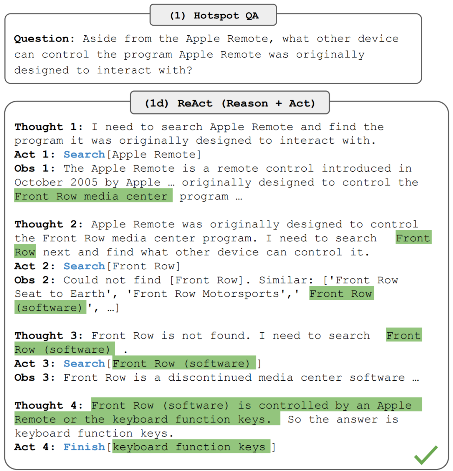
First proposed by ReAct (Yao et al., 2022), interleaving reasoning and action has become a common pattern for agents. Yao et al. used the term “reasoning” to encompass both planning and reflection. At each step, the agent is asked to explain its thinking (planning), take actions, then analyze observations (reflection), until the task is considered finished by the agent. The agent is typically prompted, using examples, to generate outputs in the following format:
Thought 1: …
Act 1: …
Observation 1: …

… [continue until reflection determines that the task is finished] …

Thought N: …
Act N: Finish [Response to query]
Figure 6-12 shows an example of an agent following the ReAct framework responding to a question from HotpotQA (Yang et al., 2018), a benchmark for multi-hop question answering.
You can implement reflection in a multi-agent setting: one agent plans and takes actions and another agent evaluates the outcome after each step or after a number of steps.
If the agent’s response failed to accomplish the task, you can prompt the agent to reflect on why it failed and how to improve. Based on this suggestion, the agent generates a new plan. This allows agents to learn from their mistakes.
For example, given a coding generation task, an evaluator might evaluate that the generated code fails ⅓ of the test cases. The agent then reflects that it failed because it didn’t take into account arrays where all numbers are negative. The actor then generates new code, taking into account all-negative arrays.
This is the approach that Reflexion (Shinn et al., 2023) took. In this framework, reflection is separated into two modules: an evaluator that evaluates the outcome and a self-reflection module that analyzes what went wrong. Figure 6-13 shows examples of Reflexion agents in action. The authors used the term “trajectory” to refer to a plan. At each step, after evaluation and self-reflection, the agent proposes a new trajectory.
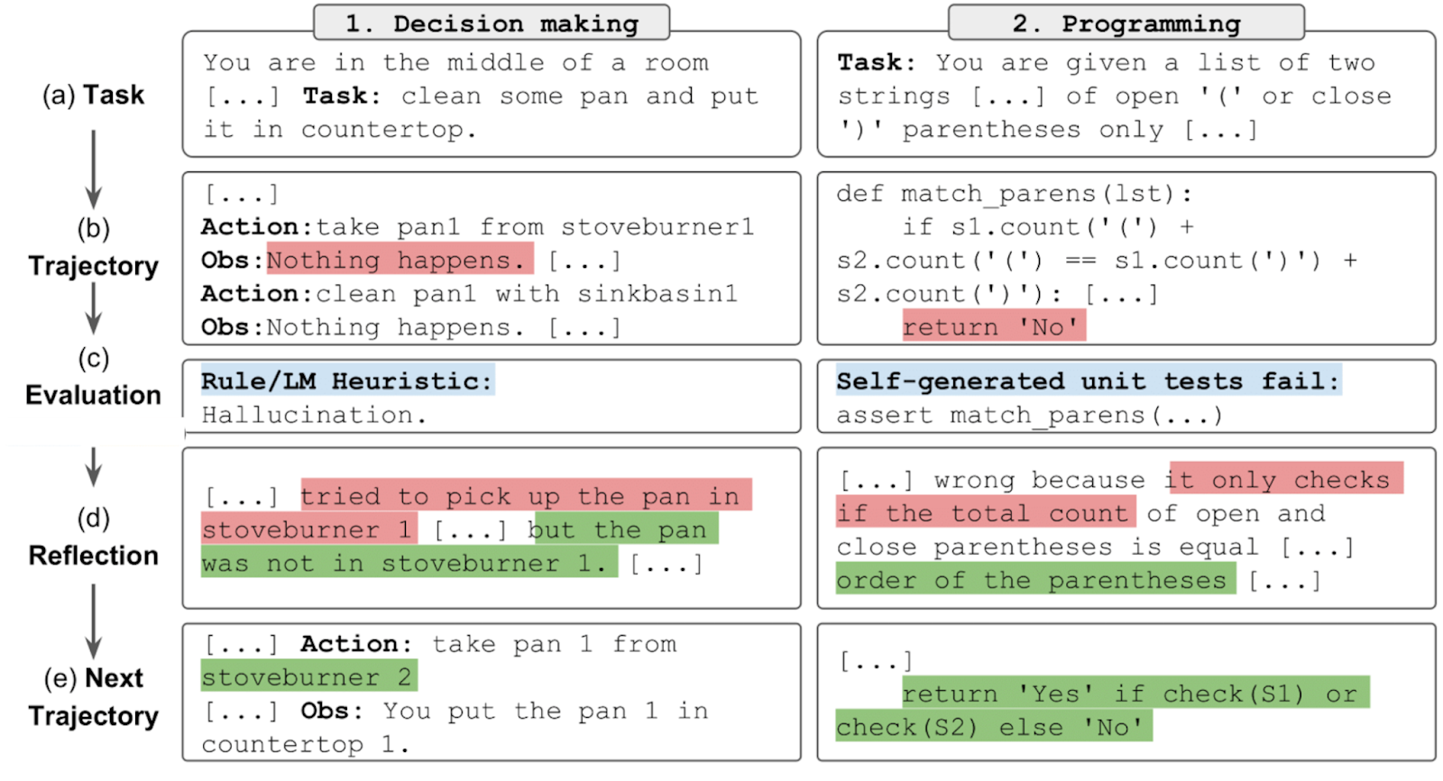
Compared to plan generation, reflection is relatively easy to implement and can bring surprisingly good performance improvement. The downside of this approach is latency and cost. Thoughts, observations, and sometimes actions can take a lot of tokens to generate, which increases cost and user-perceived latency, especially for tasks with many intermediate steps. To nudge their agents to follow the format, both ReAct and Reflexion authors used plenty of examples in their prompts. This increases the cost of computing input tokens and reduces the context space available for other information.
Because tools often play a crucial role in a task’s success, tool selection requires careful consideration. The tools to give your agent depend on the environment and the task, but also depends on the AI model that powers the agent.
There’s no foolproof guide on how to select the best set of tools. Agent literature consists of a wide range of tool inventories. For example:
More tools give the agent more capabilities. However, the more tools there are, the harder it is to efficiently use them. It’s similar to how it’s harder for humans to master a large set of tools. Adding tools also means increasing tool descriptions, which might not fit into a model’s context.
Like many other decisions while building AI applications, tool selection requires experimentation and analysis. Here are a few things you can do to help you decide:

Experiments by Chameleon (Lu et al., 2023) also demonstrate two points:
Tip:
When evaluating an agent framework, evaluate what planners and tools it supports. Different frameworks might focus on different categories of tools. For example, AutoGPT focuses on social media APIs (Reddit, X, and Wikipedia), whereas Composio focuses on enterprise APIs (Google Apps, GitHub, and Slack).
As your needs will likely change over time, evaluate how easy it is to extend your agent to incorporate new tools.
As humans, we become more productive not just by using the tools we’re given, but also by creating progressively more powerful tools from simpler ones. Can AI create new tools from its initial tools?
Chameleon (Lu et al., 2023) proposes the study of tool transition: after tool X, how likely is the agent to call tool Y? Figure 6-15 shows an example of tool transition. If two tools are frequently used together, they can be combined into a bigger tool. If an agent is aware of this information, the agent itself can combine initial tools to continually build more complex tools.
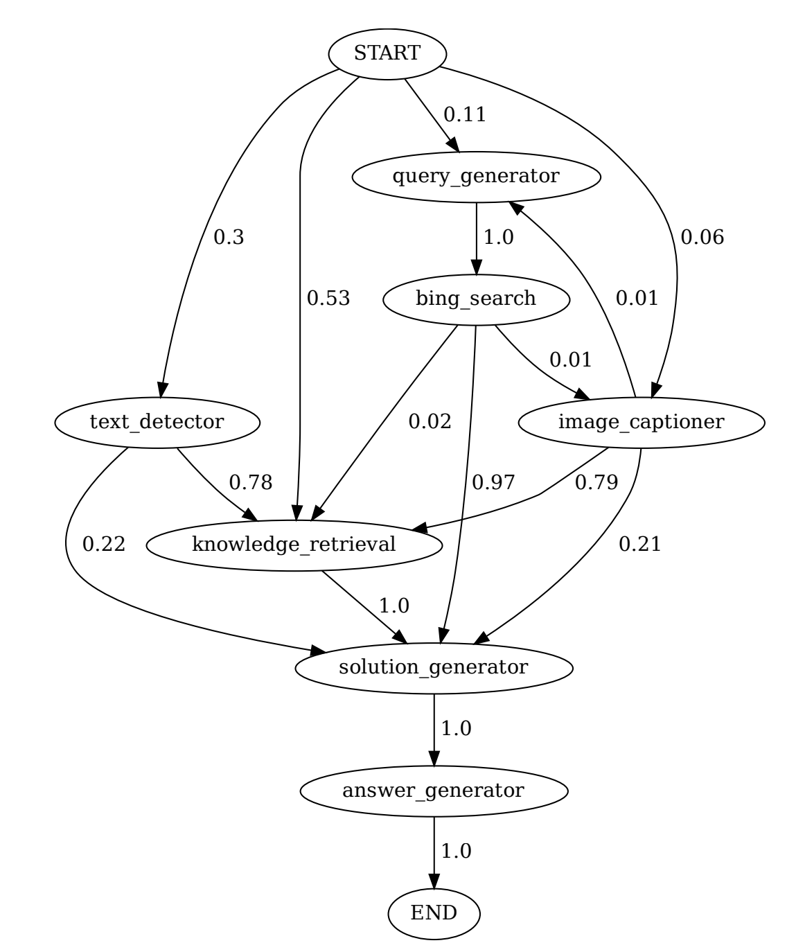
Vogager (Wang et al., 2023) proposes a skill manager to keep track of new skills (tools) that an agent acquires for later reuse. Each skill is a coding program. When the skill manager determines a newly created skill is to be useful (e.g., because it’s successfully helped an agent accomplish a task), it adds this skill to the skill library (conceptually similar to the tool inventory). This skill can be retrieved later to use for other tasks.
Earlier in this section, we mentioned that the success of an agent in an environment depends on its tool inventory and its planning capabilities. Failures in either aspect can cause the agent to fail. The next section will discuss different failure modes of an agent and how to evaluate them.
Evaluation is about detecting failures. The more complex a task an agent performs, the more possible failure points there are. Other than the failure modes common to all AI applications discussed in Chapters 3 and 4, agents also have unique failures caused by planning, tool execution, and efficiency. Some of the failures are easier to catch than others.
To evaluate an agent, identify its failure modes and measure how often each of these failure modes happens.
Planning is hard and can fail in many ways. The most common mode of planning failure is tool use failure. The agent might generate a plan with one or more of these errors.
Invalid tool
For example, it generates a plan that contains bing_search, which isn’t in the tool inventory.
Valid tool, invalid parameters.
For example, it calls lbs_to_kg with two parameters, but this function requires only one parameter, lbs.
Valid tool, incorrect parameter values
For example, it calls lbs_to_kg with one parameter, lbs, but uses the value 100 for lbs when it should be 120.
Another mode of planning failure is goal failure: the agent fails to achieve the goal. This can be because the plan doesn’t solve a task, or it solves the task without following the constraints. To illustrate this, imagine you ask the model to plan a two-week trip from San Francisco to India with a budget of $5,000. The agent might plan a trip from San Francisco to Vietnam, or plan you a two-week trip from San Francisco to India that will cost you way over the budget.
A common constraint that is often overlooked by agent evaluation is time. In many cases, the time an agent takes matters less because you can assign a task to an agent and only need to check in when it’s done. However, in many cases, the agent becomes less useful with time. For example, if you ask an agent to prepare a grant proposal and the agent finishes it after the grant deadline, the agent isn’t very helpful.
An interesting mode of planning failure is caused by errors in reflection. The agent is convinced that it’s accomplished a task when it hasn’t. For example, you ask the agent to assign 50 people to 30 hotel rooms. The agent might assign only 40 people and insist that the task has been accomplished.
To evaluate an agent for planning failures, one option is to create a planning dataset where each example is a tuple (task, tool inventory). For each task, use the agent to generate a K number of plans. Compute the following metrics:
Analyze the agent’s outputs for patterns. What types of tasks does the agent fail more on? Do you have a hypothesis why? What tools does the model frequently make mistakes with? Some tools might be harder for an agent to use. You can improve an agent’s ability to use a challenging tool by better prompting, more examples, or finetuning. If all fail, you might consider swapping out this tool for something easier to use.
Tool failures happen when the correct tool is used, but the tool output is wrong. One failure mode is when a tool just gives the wrong outputs. For example, an image captioner returns a wrong description, or an SQL query generator returns a wrong SQL query.
If the agent generates only high-level plans and a translation module is involved in translating from each planned action to executable commands, failures can happen because of translation errors.
Tool failures are tool-dependent. Each tool needs to be tested independently. Always print out each tool call and its output so that you can inspect and evaluate them. If you have a translator, create benchmarks to evaluate it.
Detecting missing tool failures requires an understanding of what tools should be used. If your agent frequently fails on a specific domain, this might be because it lacks tools for this domain. Work with human domain experts and observe what tools they would use.
An agent might generate a valid plan using the right tools to accomplish a task, but it might be inefficient. Here are a few things you might want to track to evaluate an agent’s efficiency:
You can compare these metrics with your baseline, which can be another agent or a human operator. When comparing AI agents to human agents, keep in mind that humans and AI have very different modes of operation, so what’s considered efficient for humans might be inefficient for AI and vice versa. For example, visiting 100 web pages might be inefficient for a human agent who can only visit one page at a time but trivial for an AI agent that can visit all the web pages at once.
At its core, the concept of an agent is fairly simple. An agent is defined by the environment it operates in and the set of tools it has access to. In an AI-powered agent, the AI model is the brain that leverages its tools and feedback from the environment to plan how best to accomplish a task. Access to tools makes a model vastly more capable, so the agentic pattern is inevitable.
While the concept of “agents” sounds novel, they are built upon many concepts that have been used since the early days of LLMs, including self-critique, chain-of-thought, and structured outputs.
This post covered conceptually how agents work and different components of an agent. In a future post, I’ll discuss how to evaluate agent frameworks.
The agentic pattern often deals with information that exceeds a model’s context limit. A memory system that supplements the model’s context in handling information can significantly enhance an agent’s capabilities. Since this post is already long, I’ll explore how a memory system works in a future blog post.
2024-07-25 08:00:00
After studying how companies deploy generative AI applications, I noticed many similarities in their platforms. This post outlines the common components of a generative AI platform, what they do, and how they are implemented. I try my best to keep the architecture general, but certain applications might deviate. This is what the overall architecture looks like.
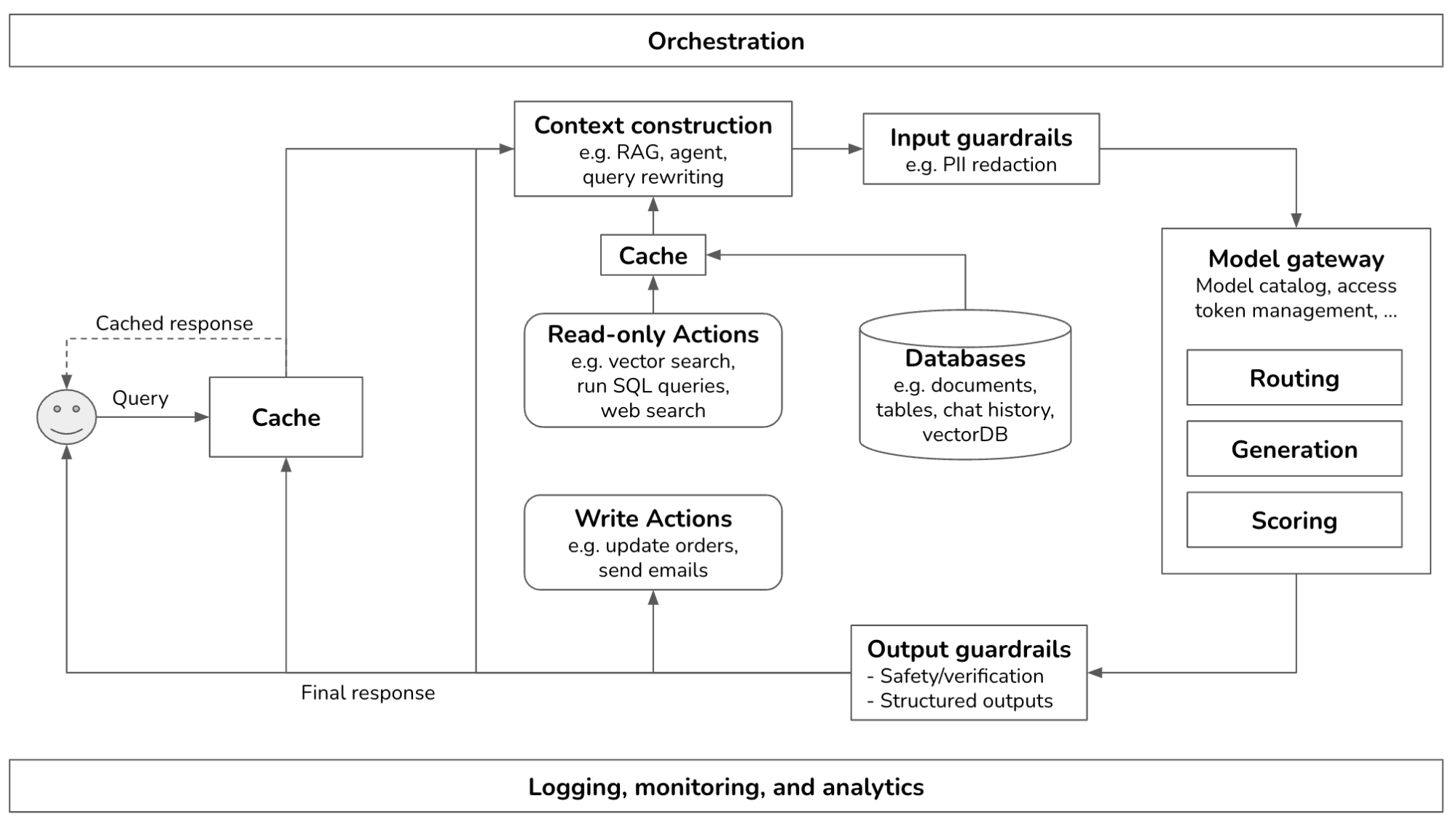
This is a pretty complex system. This post will start from the simplest architecture and progressively add more components. In its simplest form, your application receives a query and sends it to the model. The model generates a response, which is returned to the user. There are no guardrails, no augmented context, and no optimization. The Model API box refers to both third-party APIs (e.g., OpenAI, Google, Anthropic) and self-hosted APIs.
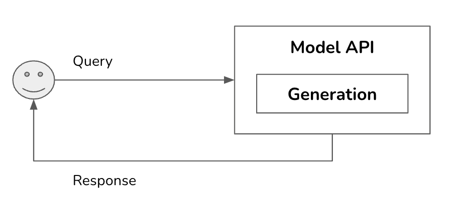
From this, you can add more components as needs arise. The order discussed in this post is common, though you don’t need to follow the exact same order. A component can be skipped if your system works well without it. Evaluation is necessary at every step of the development process.
Observability, which allows you to gain visibility into your system for monitoring and debugging, and orchestration, which involves chaining all the components together, are two essential components of the platform. We will discuss them at the end of this post.
» What this post is not «
This post focuses on the overall architecture for deploying AI applications. It discusses what components are needed and considerations when building these components. It’s not about how to build AI applications and, therefore, does NOT discuss model evaluation, application evaluation, prompt engineering, finetuning, data annotation guidelines, or chunking strategies for RAGs. All these topics are covered in my upcoming book AI Engineering.
The initial expansion of a platform usually involves adding mechanisms to allow the system to augment each query with the necessary information. Gathering the relevant information is called context construction.
Many queries require context to answer. The more relevant information there is in the context, the less the model has to rely on its internal knowledge, which can be unreliable due to its training data and training methodology. Studies have shown that having access to relevant information in the context can help the model generate more detailed responses while reducing hallucinations (Lewis et al., 2020).
For example, given the query “Will Acme’s fancy-printer-A300 print 100pps?”, the model will be able to respond better if it’s given the specifications of fancy-printer-A300. (Thanks Chetan Tekur for the example.)
Context construction for foundation models is equivalent to feature engineering for classical ML models. They serve the same purpose: giving the model the necessary information to process an input.
In-context learning, learning from the context, is a form of continual learning. It enables a model to incorporate new information continually to make decisions, preventing it from becoming outdated. For example, a model trained on last-week data won’t be able to answer questions about this week unless the new information is included in its context. By updating a model’s context with the latest information, e.g. fancy-printer-A300’s latest specifications, the model remains up-to-date and can respond to queries beyond its cut-off date.
The most well-known pattern for context construction is RAG, Retrieval-Augmented Generation. RAG consists of two components: a generator (e.g. a language model) and a retriever, which retrieves relevant information from external sources.
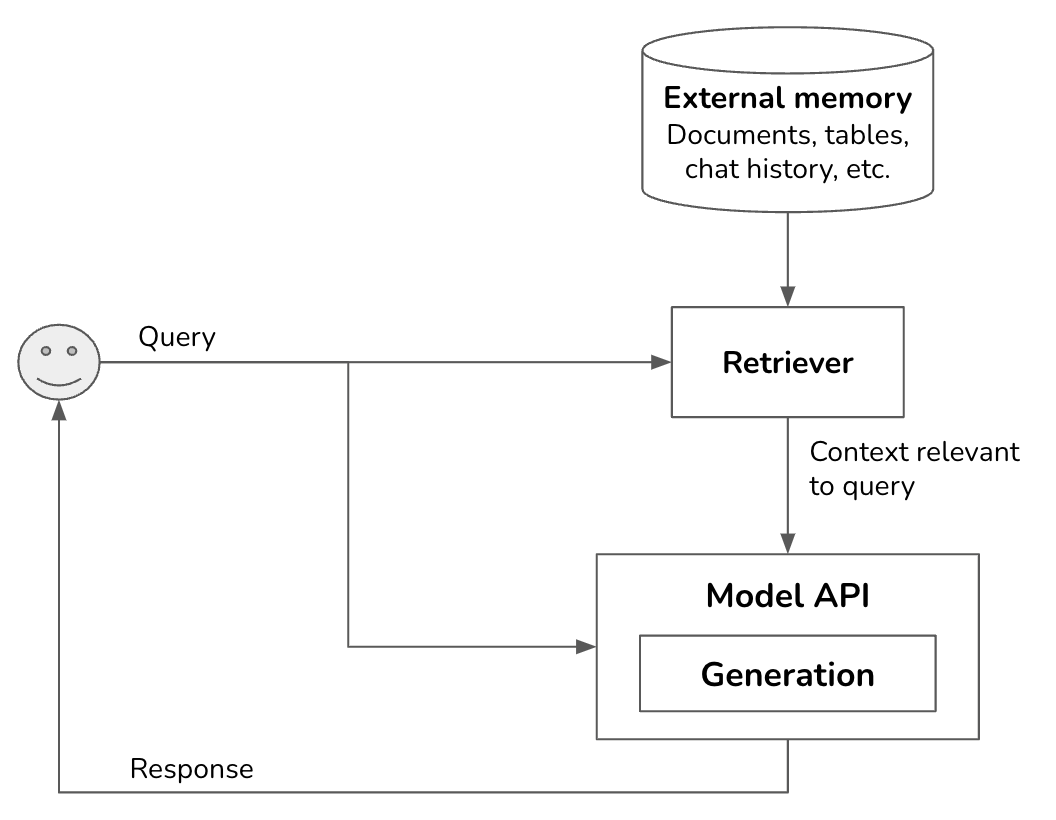
Retrieval isn’t unique to RAGs. It’s the backbone of search engines, recommender systems, log analytics, etc. Many retrieval algorithms developed for traditional retrieval systems can be used for RAGs.
External memory sources typically contain unstructured data, such as memos, contracts, news updates, etc. They can be collectively called documents. A document can be 10 tokens or 1 million tokens. Naively retrieving whole documents can cause your context to be arbitrarily long. RAG typically requires documents to be split into manageable chunks, which can be determined from the model’s maximum context length and your application’s latency requirements. To learn more about chunking and the optimal chunk size, see Pinecone, Langchain, Llamaindex, and Greg Kamradt’s tutorials.
Once data from external memory sources has been loaded and chunked, retrieval is performed using two main approaches.
Embedding-based retrieval (also known as vector search)
You convert chunks of data into embedding vectors using an embedding model such as BERT, sentence-transformers, and proprietary embedding models provided by OpenAI or Google. Given a query, the data whose vectors are closest to the query embedding, as determined by the vector search algorithm, is retrieved.
Vector search is usually framed as nearest-neighbor search, using approximate nearest neighbor (ANN) algorithms such as FAISS (Facebook AI Similarity Search), Google’s ScaNN, Spotify’s ANNOY, and hnswlib (Hierarchical Navigable Small World).
The ANN-benchmarks website compares different ANN algorithms on multiple datasets using four main metrics, taking into account the tradeoffs between indexing and querying.
This works with not just text documents, but also images, videos, audio, and code. Many teams even try to summarize SQL tables and dataframes and then use these summaries to generate embeddings for retrieval.
Term-based retrieval is much faster and cheaper than embedding-based retrieval. It can work well out of the box, making it an attractive option to start. Both BM25 and Elasticsearch are widely used in the industry and serve as formidable baselines for more complex retrieval systems. Embedding-based retrieval, while computationally expensive, can be significantly improved over time to outperform term-based retrieval.
A production retrieval system typically combines several approaches. Combining term-based retrieval and embedding-based retrieval is called hybrid search.
One common pattern is sequential. First, a cheap, less precise retriever, such as a term-based system, fetches candidates. Then, a more precise but more expensive mechanism, such as k-nearest neighbors, finds the best of these candidates. The second step is also called reranking.
For example, given the term “transformer”, you can fetch all documents that contain the word transformer, regardless of whether they are about the electric device, the neural architecture, or the movie. Then you use vector search to find among these documents those that are actually related to your transformer query.
Context reranking differs from traditional search reranking in that the exact position of items is less critical. In search, the rank (e.g., first or fifth) is crucial. In context reranking, the order of documents still matters because it affects how well a model can process them. Models might better understand documents at the beginning and end of the context, as suggested by the paper Lost in the middle (Liu et al., 2023). However, as long as a document is included, the impact of its order is less significant compared to in search ranking.
Another pattern is ensemble. Remember that a retriever works by ranking documents by their relevance scores to the query. You use multiple retrievers to fetch candidates at the same time, then combine these different rankings together to generate a final ranking.
External data sources can also be structured, such as dataframes or SQL tables. Retrieving data from an SQL table is significantly different from retrieving data from unstructured documents. Given a query, the system works as follows.
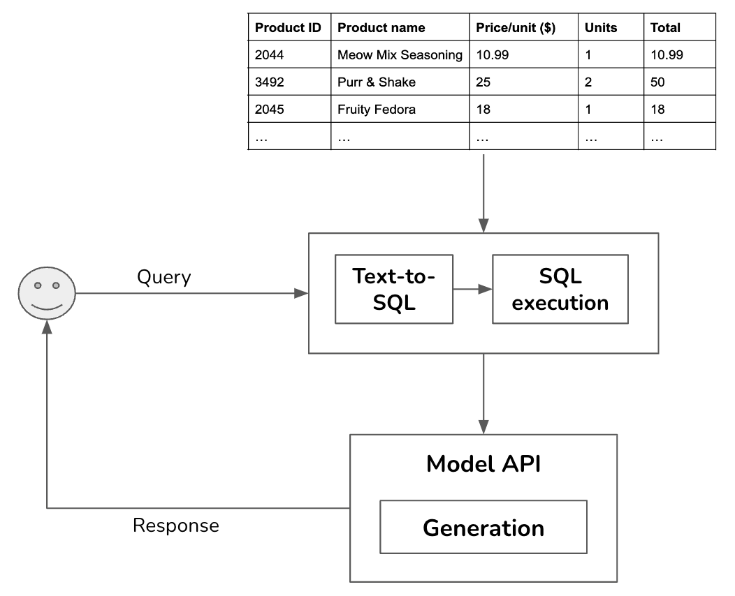
For the text-to-SQL step, if there are many available tables whose schemas can’t all fit into the model context, you might need an intermediate step to predict what tables to use for each query. Text-to-SQL can be done by the same model used to generate the final response or one of many specialized text-to-SQL models.
An important source of data is the Internet. A web search tool like Google or Bing API can give the model access to a rich, up-to-date resource to gather relevant information for each query. For example, given the query “Who won Oscar this year?”, the system searches for information about the latest Oscar and uses this information to generate the final response to the user.
Term-based retrieval, embedding-based retrieval, SQL execution, and web search are actions that a model can take to augment its context. You can think of each action as a function the model can call. A workflow that can incorporate external actions is also called agentic. The architecture then looks like this.
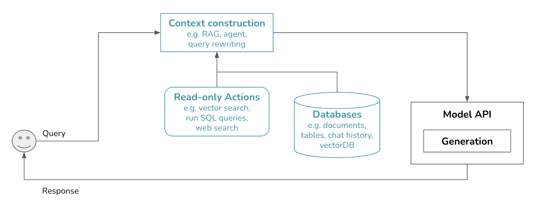
» Action vs. tool «
A tool allows one or more actions. For example, a people search tool might allow two actions: search by name and search by email. However, the difference is minimal, so many people use action and tool interchangeably.
» Read-only actions vs. write actions «
Actions that retrieve information from external sources but don’t change their states are read-only actions. Giving a model write actions, e.g. updating the values in a table, enables the model to perform more tasks but also poses more risks, which will be discussed later.
Often, a user query needs to be rewritten to increase the likelihood of fetching the right information. Consider the following conversation.
User: When was the last time John Doe bought something from us?
AI: John last bought a Fruity Fedora hat from us two weeks ago, on January 3, 2030.
User: How about Emily Doe?
The last question, “How about Emily Doe?”, is ambiguous. If you use this query verbatim to retrieve documents, you’ll likely get irrelevant results. You need to rewrite this query to reflect what the user is actually asking. The new query should make sense on its own. The last question should be rewritten to “When was the last time Emily Doe bought something from us?”
Query rewriting is typically done using other AI models, using a prompt similar to “Given the following conversation, rewrite the last user input to reflect what the user is actually asking.”
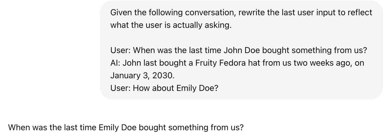
Query rewriting can get complicated, especially if you need to do identity resolution or incorporate other knowledge. If the user asks “How about his wife?”, you will first need to query your database to find out who his wife is. If you don’t have this information, the rewriting model should acknowledge that this query isn’t solvable instead of hallucinating a name, leading to a wrong answer.
Guardrails help reduce AI risks and protect not just your users but also you, the developers. They should be placed whenever there is potential for failures. This post discusses two types of guardrails: input guardrails and output guardrails.
Input guardrails are typically protection against two types of risks: leaking private information to external APIs, and executing bad prompts that compromise your system (model jailbreaking).
This risk is specific to using external model APIs when you need to send your data outside your organization. For example, an employee might copy the company’s secret or a user’s private information into a prompt and send it to wherever the model is hosted.
One of the most notable early incidents was when Samsung employees put Samsung’s proprietary information into ChatGPT, accidentally leaking the company’s secrets. It’s unclear how Samsung discovered this leak and how the leaked information was used against Samsung. However, the incident was serious enough for Samsung to ban ChatGPT in May 2023.
There’s no airtight way to eliminate potential leaks when using third-party APIs. However, you can mitigate them with guardrails. You can use one of the many available tools that automatically detect sensitive data. What sensitive data to detect is specified by you. Common sensitive data classes are:
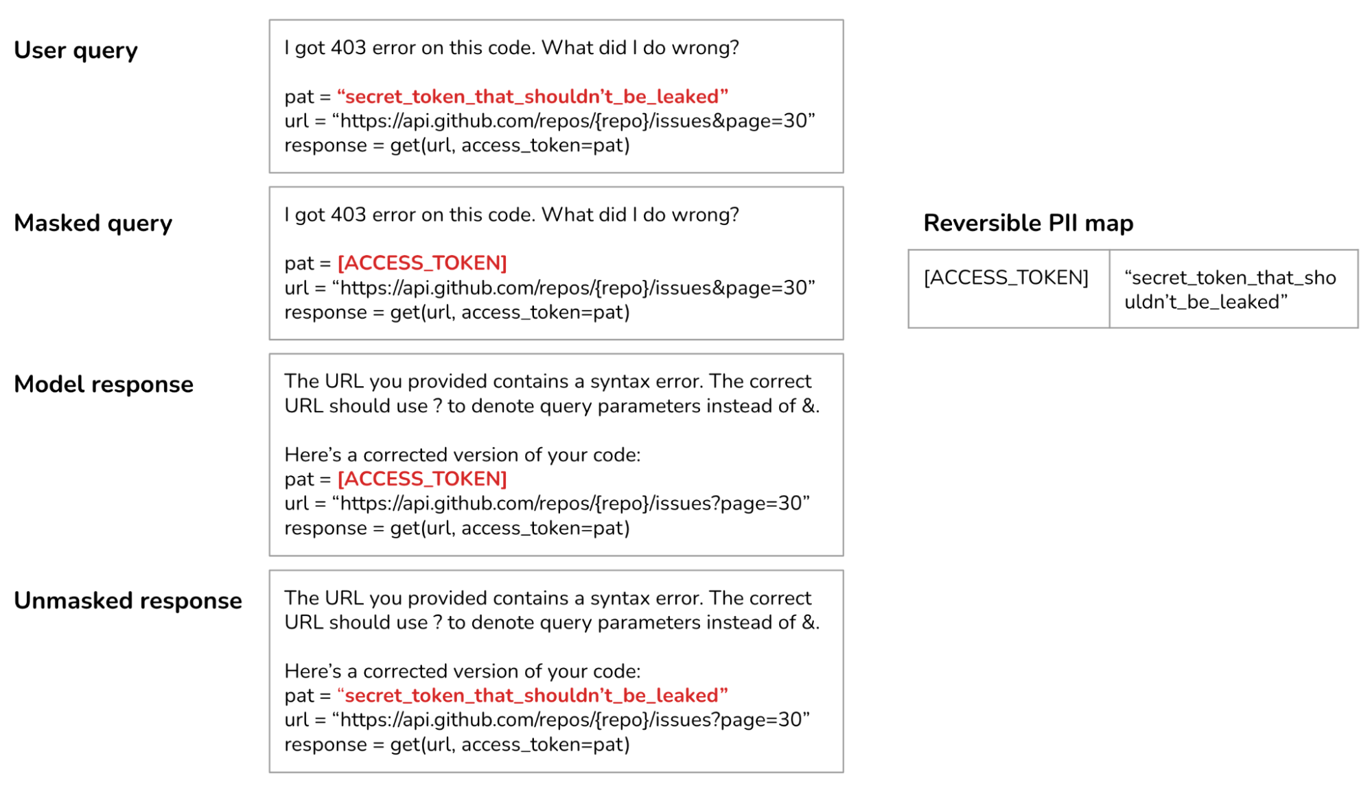
Many sensitive data detection tools use AI to identify potentially sensitive information, such as determining if a string resembles a valid home address. If a query is found to contain sensitive information, you have two options: block the entire query or remove the sensitive information from it. For instance, you can mask a user’s phone number with the placeholder [PHONE NUMBER]. If the generated response contains this placeholder, use a PII reversible dictionary that maps this placeholder to the original information so that you can unmask it, as shown below.
It’s become an online sport to try to jailbreak AI models, getting them to say or do bad things. While some might find it amusing to get ChatGPT to make controversial statements, it’s much less fun if your customer support chatbot, branded with your name and logo, does the same thing. This can be especially dangerous for AI systems that have access to tools. Imagine if a user finds a way to get your system to execute an SQL query that corrupts your data.
To combat this, you should first put guardrails on your system so that no harmful actions can be automatically executed. For example, no SQL queries that can insert, delete, or update data can be executed without human approval. The downside of this added security is that it can slow down your system.
To prevent your application from making outrageous statements it shouldn’t be making, you can define out-of-scope topics for your application. For example, if your application is a customer support chatbot, it shouldn’t answer political or social questions. A simple way to do so is to filter out inputs that contain predefined phrases typically associated with controversial topics, such as “immigration” or “antivax”. More sophisticated algorithms use AI to classify whether an input is about one of the pre-defined restricted topics.
If harmful prompts are rare in your system, you can use an anomaly detection algorithm to identify unusual prompts.
AI models are probabilistic, making their outputs unreliable. You can put in guardrails to significantly improve your application’s reliability. Output guardrails have two main functionalities:
To catch outputs that fail to meet your standards, you need to understand what failures look like. Here are examples of failure modes and how to catch them.
Empty responses.
Malformatted responses that don’t follow the expected output format. For example, if the application expects JSON and the generated response has a missing closing bracket. There are validators for certain formats, such as regex, JSON, and Python code validators. There are also tools for constrained sampling such as guidance, outlines, and instructor.
Toxic responses, such as those that are racist or sexist. These responses can be caught using one of many toxicity detection tools.
Factual inconsistent responses hallucinated by the model. Hallucination detection is an active area of research with solutions such as SelfCheckGPT (Manakul et al., 2023) and SAFE, Search Engine Factuality Evaluator (Wei et al., 2024). You can mitigate hallucinations by providing models with sufficient context and prompting techniques such as chain-of-thought. Hallucination detection and mitigation are discussed further in my upcoming book AI Engineering.
This failure mode can be prevented by not training your model on sensitive data and not allowing it to retrieve sensitive data in the first place. Sensitive data in outputs can be detected using the same tools used for input guardrails.
Brand-risk responses, such as responses that mischaracterize your company or your competitors. An example is when Grok, a model trained by X, generated a response suggesting that Grok was trained by OpenAI, causing the Internet to suspect X of stealing OpenAI’s data. This failure mode can be mitigated with keyword monitoring. Once you’ve identified outputs concerning your brands and competitors, you can either block these outputs, pass them onto human reviewers, or use other models to detect the sentiment of these outputs to ensure that only the right sentiments are returned.
AI models are probabilistic, which means that if you try a query again, you might get a different response. Many failures can be mitigated using a basic retry logic. For example, if the response is empty, try again X times or until you get a non-empty response. Similarly, if the response is malformatted, try again until the model generates a correctly formatted response.
This retry policy, however, can incur extra latency and cost. One retry means 2x the number of API calls. If the retry is carried out after failure, the latency experienced by the user will double. To reduce latency, you can make calls in parallel. For example, for each query, instead of waiting for the first query to fail before retrying, you send this query to the model twice at the same time, get back two responses, and pick the better one. This increases the number of redundant API calls but keeps latency manageable.
It’s also common to fall back on humans to handle tricky queries. For example, you can transfer a query to human operators if it contains specific key phrases. Some teams use a specialized model, potentially trained in-house, to decide when to transfer a conversation to humans. One team, for instance, transfers a conversation to human operators when their sentiment analysis model detects that the user is getting angry. Another team transfers a conversation after a certain number of turns to prevent users from getting stuck in an infinite loop.
Reliability vs. latency tradeoff: While acknowledging the importance of guardrails, some teams told me that latency is more important. They decided not to implement guardrails because they can significantly increase their application’s latency. However, these teams are in the minority. Most teams find that the increased risks are more costly than the added latency.
Output guardrails might not work well in the stream completion mode. By default, the whole response is generated before shown to the user, which can take a long time. In the stream completion mode, new tokens are streamed to the user as they are generated, reducing the time the user has to wait to see the response. The downside is that it’s hard to evaluate partial responses, so unsafe responses might be streamed to users before the system guardrails can determine that they should be blocked.
Self-hosted vs. third-party API tradeoff: Self-hosting your models means that you don’t have to send your data to a third party, reducing the need for input guardrails. However, it also means that you must implement all the necessary guardrails yourself, rather than relying on the guardrails provided by third-party services.
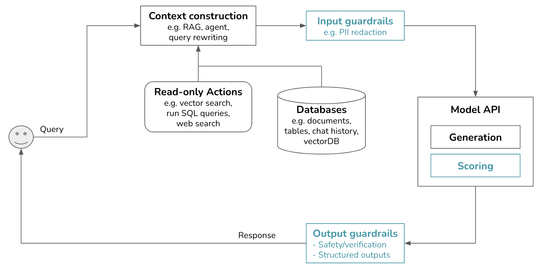
Our platform now looks like this. Guardrails can be independent tools or parts of model gateways, as discussed later. Scorers, if used, are grouped under model APIs since scorers are typically AI models, too. Models used for scoring are typically smaller and faster than models used for generation.
As applications grow in complexity and involve more models, two types of tools emerged to help you work with multiple models: routers and gateways.
An application can use different models to respond to different types of queries. Having different solutions for different queries has several benefits. First, this allows you to have specialized solutions, such as one model specialized in technical troubleshooting and another specialized in subscriptions. Specialized models can potentially perform better than a general-purpose model. Second, this can help you save costs. Instead of routing all queries to an expensive model, you can route simpler queries to cheaper models.
A router typically consists of an intent classifier that predicts what the user is trying to do. Based on the predicted intent, the query is routed to the appropriate solution. For example, for a customer support chatbot, if the intent is:
An intent classifier can also help your system avoid out-of-scope conversations. For example, you can have an intent classifier that predicts whether a query is out of the scope. If the query is deemed inappropriate (e.g. if the user asks who you would vote for in the upcoming election), the chatbot can politely decline to engage using one of the stock responses (“As a chatbot, I don’t have the ability to vote. If you have questions about our products, I’d be happy to help.”) without wasting an API call.
If your system has access to multiple actions, a router can involve a next-action predictor to help the system decide what action to take next. One valid action is to ask for clarification if the query is ambiguous. For example, in response to the query “Freezing,” the system might ask, “Do you want to freeze your account or are you talking about the weather?” or simply say, “I’m sorry. Can you elaborate?”
Intent classifiers and next-action predictors can be general-purpose models or specialized classification models. Specialized classification models are typically much smaller and faster than general-purpose models, allowing your system to use multiple of them without incurring significant extra latency and cost.
When routing queries to models with varying context limits, the query’s context might need to be adjusted accordingly. Consider a query of 1,000 tokens that is slated for a model with a 4K context limit. The system then takes an action, e.g. web search, that brings back 8,000-token context. You can either truncate the query’s context to fit the originally intended model or route the query to a model with a larger context limit.
A model gateway is an intermediate layer that allows your organization to interface with different models in a unified and secure manner. The most basic functionality of a model gateway is to enable developers to access different models – be it self-hosted models or models behind commercial APIs such as OpenAI or Google – the same way. A model gateway makes it easier to maintain your code. If a model API changes, you only need to update the model gateway instead of having to update all applications that use this model API.
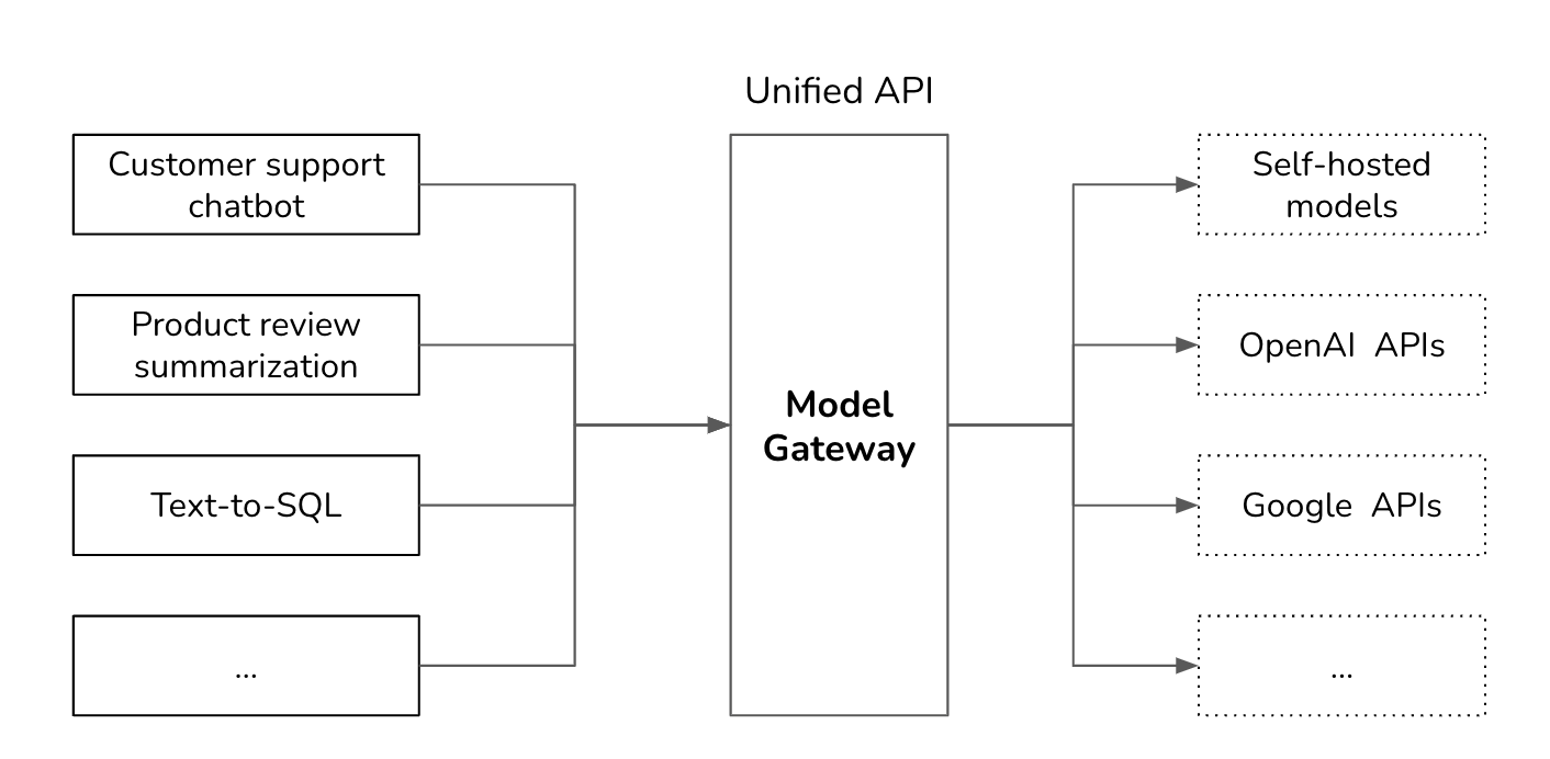
In its simplest form, a model gateway is a unified wrapper that looks like the following code example. This example is to give you an idea of how a model gateway might be implemented. It’s not meant to be functional as it doesn’t contain any error checking or optimization.
import google.generativeai as genai
import openai

def openai_model(input_data, model_name, max_tokens):
    openai.api_key = os.environ["OPENAI_API_KEY"]
    response = openai.Completion.create(
        engine=model_name,
        prompt=input_data,
        max_tokens=max_tokens
    )
    return {"response": response.choices[0].text.strip()}

def gemini_model(input_data, model_name, max_tokens):
    genai.configure(api_key=os.environ["GOOGLE_API_KEY"])
    model = genai.GenerativeModel(model_name=model_name)
    response = model.generate_content(input_data, max_tokens=max_tokens)
    return {"response": response["choices"][0]["message"]["content"]}

@app.route('/model', methods=['POST'])
def model_gateway():
    data = request.get_json()
    model_type = data.get("model_type")
    model_name = data.get("model_name")
    input_data = data.get("input_data")
    max_tokens = data.get("max_tokens")

    if model_type == "openai":
        result = openai_model(input_data, model_name, max_tokens)
    elif model_type == "gemini":
        result = gemini_model(input_data, model_name, max_tokens)
    return jsonify(result)
A model gateway is access control and cost management. Instead of giving everyone who wants access to the OpenAI API your organizational tokens, which can be easily leaked, you only give people access to the model gateway, creating a centralized and controlled point of access. The gateway can also implement fine-grained access controls, specifying which user or application should have access to which model. Moreover, the gateway can monitor and limit the usage of API calls, preventing abuse and managing costs effectively.
A model gateway can also be used to implement fallback policies to overcome rate limits or API failures (the latter is unfortunately common). When the primary API is unavailable, the gateway can route requests to alternative models, retry after a short wait, or handle failures in other graceful manners. This ensures that your application can operate smoothly without interruptions.
Since requests and responses are already flowing through the gateway, it’s a good place to implement other functionalities such as load balancing, logging, and analytics. Some gateway services even provide caching and guardrails.
Given that gateways are relatively straightforward to implement, there are many off-the-shelf gateways. Examples include Portkey’s gateway, MLflow AI Gateway, WealthSimple’s llm-gateway, TrueFoundry, Kong, and Cloudflare.
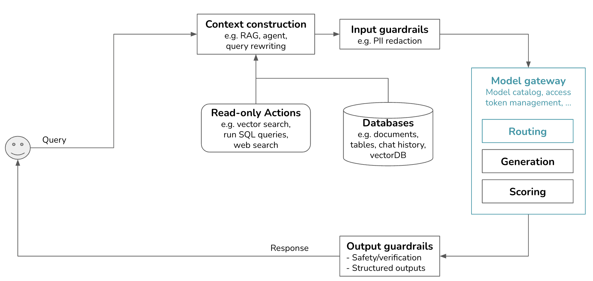
With the added gateway and routers, our platform is getting more exciting. Like scoring, routing is also in the model gateway. Like models used for scoring, models used for routing are typically smaller than models used for generation.
When I shared this post with my friend Eugene Yan, he said that cache is perhaps the most underrated component of an AI platform. Caching can significantly reduce your application’s latency and cost.
Cache techniques can also be used during training, but since this post is about deployment, I’ll focus on cache for inference. Some common inference caching techniques include prompt cache, exact cache, and semantic cache. Prompt cache are typically implemented by the inference APIs that you use. When evaluating an inference library, it’s helpful to understand what cache mechanism it supports.
KV cache for the attention mechanism is out of scope for this discussion.
Many prompts in an application have overlapping text segments. For example, all queries can share the same system prompt. A prompt cache stores these overlapping segments for reuse, so you only need to process them once. A common overlapping text segment in different prompts is the system prompt. Without prompt cache, your model needs to process the system prompt with every query. With prompt cache, it only needs to process the system prompt once for the first query.
For applications with long system prompts, prompt cache can significantly reduce both latency and cost. If your system prompt is 1000 tokens and your application generates 1 million model API calls today, a prompt cache will save you from processing approximately 1 billion repetitive input tokens a day! However, this isn’t entirely free. Like KV cache, prompt cache size can be quite large and require significant engineering effort.
Prompt cache is also useful for queries that involve long documents. For example, if many of your user queries are related to the same long document (such as a book or a codebase), this long document can be cached for reuse across queries.
Since its introduction in November 2023 by Gim et al., prompt cache has already been incorporated into model APIs. Google announced that Gemini APIs will offer this functionality in June 2024 under the name context cache. Cached input tokens are given a 75% discount compared to regular input tokens, but you’ll have to pay extra for cache storage (as of writing, $1.00 / 1 million tokens per hour). Given the obvious benefits of prompt cache, I wouldn’t be surprised if it becomes as popular as KV cache.
While llama.cpp also has prompt cache, it seems to only cache whole prompts and work for queries in the same chat session. Its documentation is limited, but my guess from reading the code is that in a long conversation, it caches the previous messages and only processes the newest message.
If prompt cache and KV cache are unique to foundation models, exact cache is more general and straightforward. Your system stores processed items for reuse later when the exact items are requested. For example, if a user asks a model to summarize a product, the system checks the cache to see if a summary of this product is cached. If yes, fetch this summary. If not, summarize the product and cache the summary.
Exact cache is also used for embedding-based retrieval to avoid redundant vector search. If an incoming query is already in the vector search cache, fetch the cached search result. If not, perform a vector search for this query and cache the result.
Cache is especially appealing for queries that require multiple steps (e.g. chain-of-thought) and/or time-consuming actions (e.g. retrieval, SQL execution, or web search).
An exact cache can be implemented using in-memory storage for fast retrieval. However, since in-memory storage is limited, a cache can also be implemented using databases like PostgreSQL, Redis, or tiered storage to balance speed and storage capacity. Having an eviction policy is crucial to manage the cache size and maintain performance. Common eviction policies include Least Recently Used (LRU), Least Frequently Used (LFU), and First In, First Out (FIFO).
How long to cache a query depends on how likely this query is to be called again. User-specific queries such as “What’s the status of my recent order” are less likely to be reused by other users, and therefore, shouldn’t be cached. Similarly, it makes less sense to cache time-sensitive queries such as “How’s the weather?” Some teams train a small classifier to predict whether a query should be cached.
Unlike exact cache, semantic cache doesn’t require the incoming query to be identical to any of the cached queries. Semantic cache allows the reuse of similar queries. Imagine one user asks “What’s the capital of Vietnam?” and the model generates the answer “Hanoi”. Later, another user asks “What’s the capital city of Vietnam?”, which is the same question but with the extra word “city”. The idea of semantic cache is that the system can reuse the answer “Hanoi” instead of computing the new query from scratch.
Semantic cache only works if you have a reliable way to determine if two queries are semantically similar. One common approach is embedding-based similarity, which works as follows:
This approach requires a vector database to store the embeddings of cached queries.
Compared to other caching techniques, semantic cache’s value is more dubious because many of its components are prone to failure. Its success relies on high-quality embeddings, functional vector search, and a trustworthy similarity metric. Setting the right similarity threshold can also be tricky and require a lot of trial and error. If the system mistakes the incoming query as being similar to another query, the returned response, fetched from the cache, will be incorrect.
In addition, semantic cache can be time-consuming and compute-intensive, as it involves a vector search. The speed and cost of this vector search depend on the size of your database of cached embeddings.
Semantic cache might still be worth it if the cache hit rate is high, meaning that a good portion of queries can be effectively answered by leveraging the cached results. However, before incorporating the complexities of semantic cache, make sure to evaluate the efficiency, cost, and performance risks associated with it.
With the added cache systems, the platform looks as follows. KV cache and prompt cache are typically implemented by model API providers, so they aren’t shown in this image. If I must visualize them, I’d put them in the Model API box. There’s a new arrow to add generated responses to the cache.
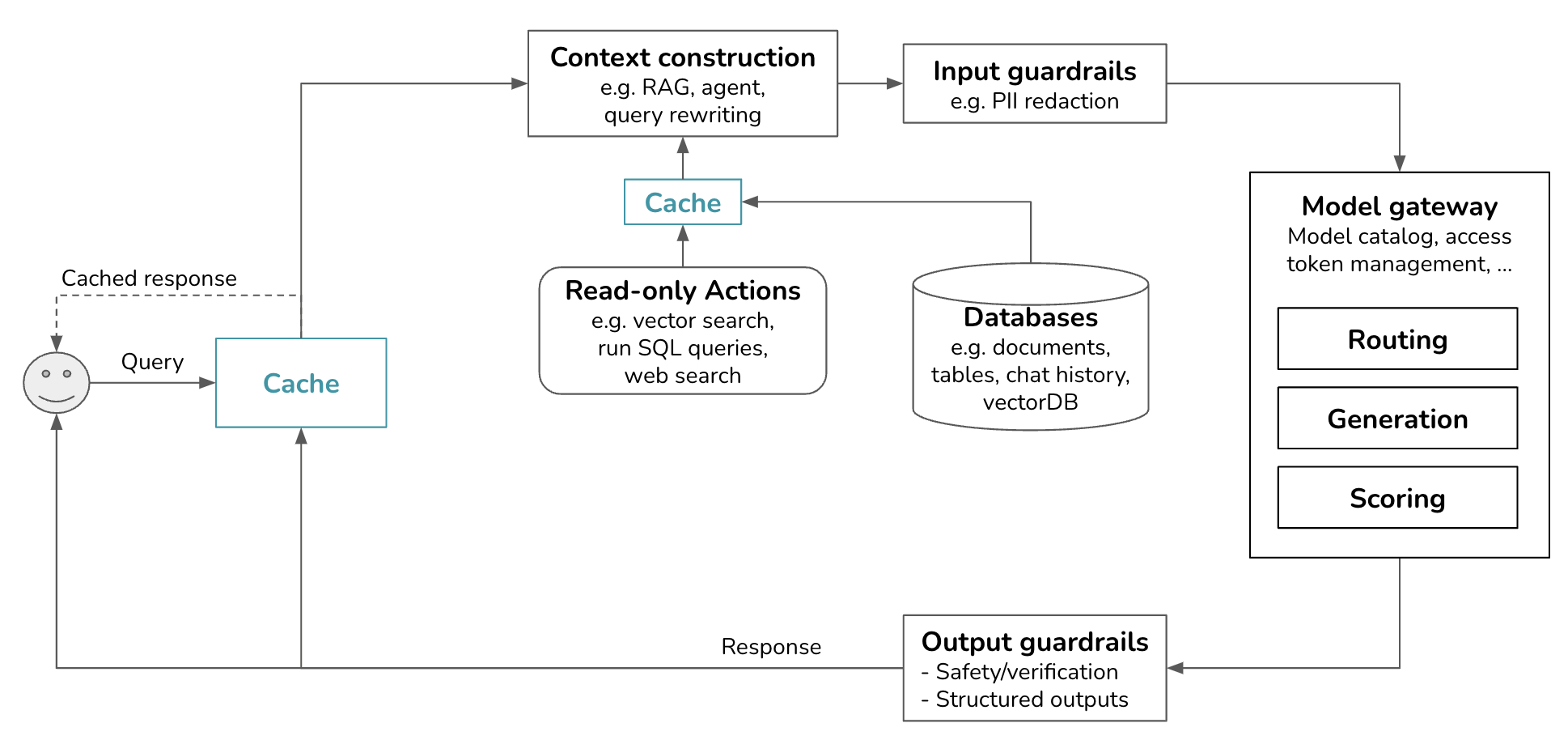
The applications we’ve discussed so far have fairly simple flows. The outputs generated by foundation models are mostly returned to users (unless they don’t pass the guardrails). However, an application flow can be more complex with loops and conditional branching. A model’s outputs can also be used to invoke write actions, such as composing an email or placing an order.
Outputs from a model can be conditionally passed onto another model or fed back to the same model as part of the input to the next step. This goes on until a model in the system decides that the task has been completed and that a final response should be returned to the user.
This can happen when you give your system the ability to plan and decide what to do next. As an example, consider the query “Plan a weekend itinerary for Paris.” The model might first generate a list of potential activities: visiting the Eiffel Tower, having lunch at a café, touring the Louvre, etc. Each of these activities can then be fed back into the model to generate more detailed plans. For instance, “visiting the Eiffel Tower” could prompt the model to generate sub-tasks like checking the opening hours, buying tickets, and finding nearby restaurants. This iterative process continues until a comprehensive and detailed itinerary is created.
Our infrastructure now has an arrow pointing the generated response back to context construction, which in turn feeds back to models in the model gateway.
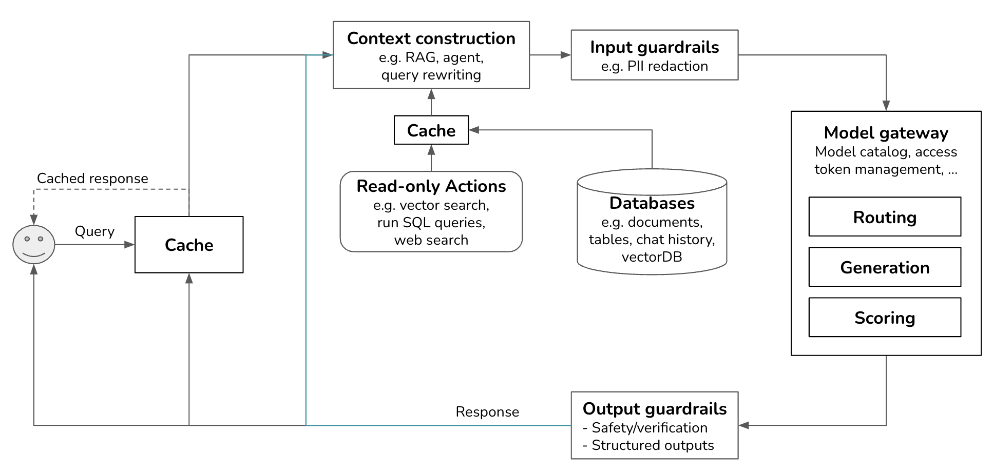
Actions used for context construction are read-only actions. They allow a model to read from its data sources to gather context. But a system can also write actions, making changes to the data sources and the world. For example, if the model outputs: “send an email to X with the message Y”, the system will invoke the action send_email(recipient=X, message=Y).
Write actions make a system vastly more capable. They can enable you to automate the whole customer outreach workflow: researching potential customers, finding their contacts, drafting emails, sending first emails, reading responses, following up, extracting orders, updating your databases with new orders, etc.
However, the prospect of giving AI the ability to automatically alter our lives is frightening. Just as you shouldn’t give an intern the authority to delete your production database, you shouldn’t allow an unreliable AI to initiate bank transfers. Trust in the system’s capabilities and its security measures is crucial. You need to ensure that the system is protected from bad actors who might try to manipulate it into performing harmful actions.
AI systems are vulnerable to cyber attacks like other software systems, but they also have another weakness: prompt injection. Prompt injection happens when an attacker manipulates input prompts into a model to get it to express undesirable behaviors. You can think of prompt injection as social engineering done on AI instead of humans.
A scenario that many companies fear is that they give an AI system access to their internal databases, and attackers trick this system into revealing private information from these databases. If the system has write access to these databases, attackers can trick the system into corrupting the data.
Any organization that wants to leverage AI needs to take safety and security seriously. However, these risks don’t mean that AI systems should never be given the ability to act in the real world. AI systems can fail, but humans can fail too. If we can get people to trust a machine to take us up into space, I hope that one day, securities will be sufficient for us to trust autonomous AI systems.
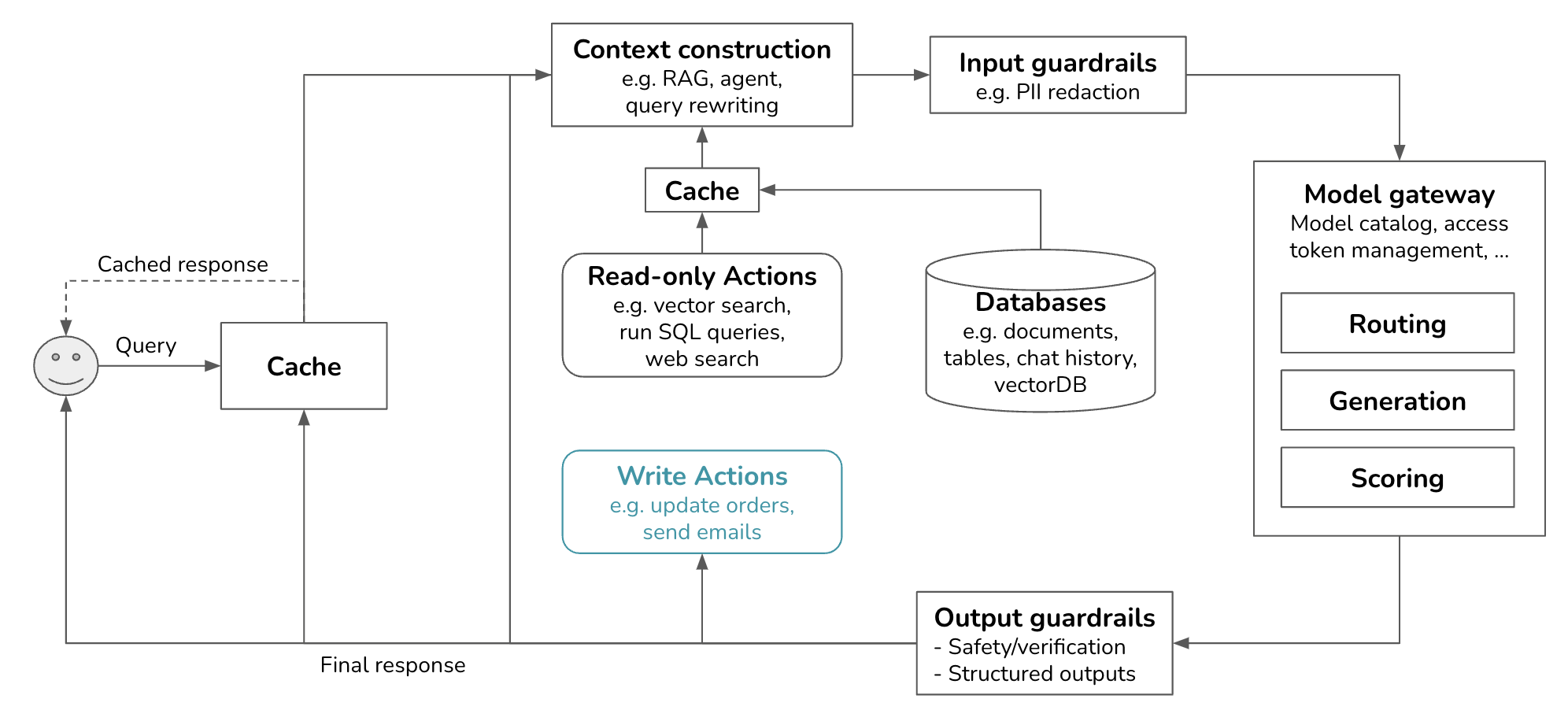
While I have placed observability in its own section, it should be integrated into the platform from the beginning rather than added later as an afterthought. Observability is crucial for projects of all sizes, and its importance grows with the complexity of the system.
This section provides the least information compared to the others. It’s impossible to cover all the nuances of observability in a blog post. Therefore, I will only give a brief overview of the three pillars of monitoring: logs, traces, and metrics. I won’t go into specifics or cover user feedback, drift detection, and debugging.
When discussing monitoring, most people think of metrics. What metrics to track depends on what you want to track about your system, which is application-specific. However, in general, there are two types of metrics you want to track: model metrics and system metrics.
System metrics tell you the state of your overall system. Common metrics are throughput, memory usage, hardware utilization, and service availability/uptime. System metrics are common to all software engineering applications. In this post, I’ll focus on model metrics.
Model metrics assess your model’s performance, such as accuracy, toxicity, and hallucination rate. Different steps in an application pipeline also have their own metrics. For example, in a RAG application, the retrieval quality is often evaluated using context relevance and context precision. A vector database can be evaluated by how much storage it needs to index the data and how long it takes to query the data
There are various ways a model’s output can fail. It’s crucial to identify these issues and develop metrics to monitor them. For example, you might want to track how often your model times out, returns empty responses or produces malformatted responses. If you’re worried about your model revealing sensitive information, find a way to track that too.
Length-related metrics such as query, context, and response length are helpful for understanding your model’s behaviors. Is one model more verbose than another? Are certain types of queries more likely to result in lengthy answers? They are especially useful for detecting changes in your application. If the average query length suddenly decreases, it could indicate an underlying issue that needs investigation.
Length-related metrics are also important for tracking latency and costs, as longer contexts and responses typically increase latency and incur higher costs.
Tracking latency is essential for understanding the user experience. Common latency metrics include:
You’ll also want to track costs. Cost-related metrics are the number of queries and the volume of input and output tokens. If you use an API with rate limits, tracking the number of requests per second is important to ensure you stay within your allocated limits and avoid potential service interruptions.
When calculating metrics, you can choose between spot checks and exhaustive checks. Spot checks involve sampling a subset of data to quickly identify issues, while exhaustive checks evaluate every request for a comprehensive performance view. The choice depends on your system’s requirements and available resources, with a combination of both providing a balanced monitoring strategy.
When computing metrics, ensure they can be broken down by relevant axes, such as users, releases, prompt/chain versions, prompt/chain types, and time. This granularity helps in understanding performance variations and identifying specific issues.
Since this blog post is getting long and I’ve written at length about logs in Designing Machine Learning Systems, I will be quick here. The philosophy for logging is simple: log everything. Log the system configurations. Log the query, the output, and the intermediate outputs. Log when a component starts, ends, when something crashes, etc. When recording a piece of log, make sure to give it tags and IDs that can help you know where in the system this log comes from.
Logging everything means that the amount of logs you have can grow very quickly. Many tools for automated log analysis and log anomaly detection are powered by AI.
While it’s impossible to manually process logs, it’s useful to manually inspect your production data daily to get a sense of how users are using your application. Shankar et al. (2024) found that the developers’ perceptions of what constitutes good and bad outputs change as they interact with more data, allowing them to both rewrite their prompts to increase the chance of good responses and update their evaluation pipeline to catch bad responses.
Trace refers to the detailed recording of a request’s execution path through various system components and services. In an AI application, tracing reveals the entire process from when a user sends a query to when the final response is returned, including the actions the system takes, the documents retrieved, and the final prompt sent to the model. It should also show how much time each step takes and its associated cost, if measurable. As an example, this is a visualization of a Langsmith trace.
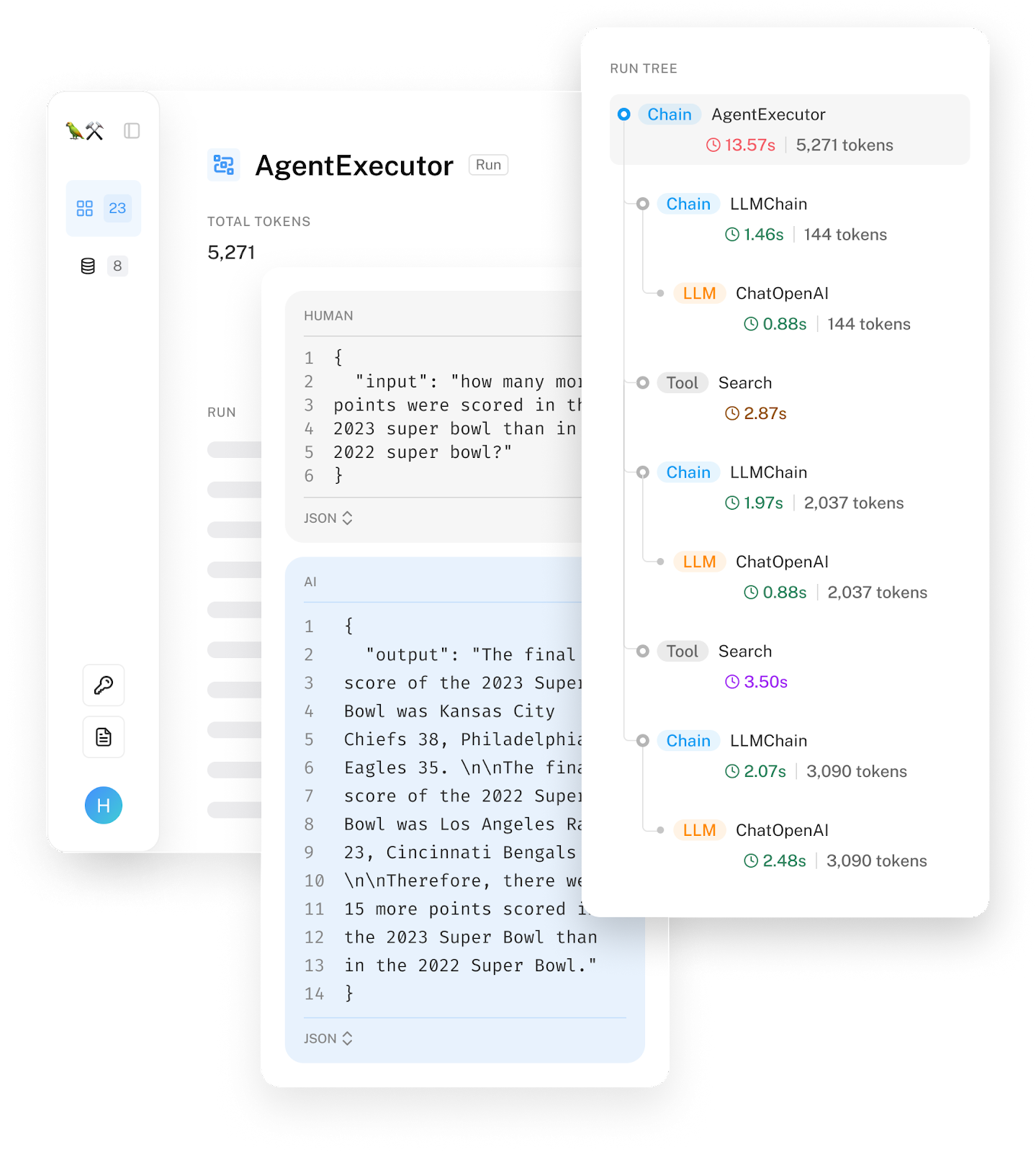
Ideally, you should be able to trace each query’s transformation through the system step-by-step. If a query fails, you should be able to pinpoint the exact step where it went wrong: whether it was incorrectly processed, the retrieved context was irrelevant, or the model generated a wrong response.
An AI application can get fairly complex, consisting of multiple models, retrieving data from many databases, and having access to a wide range of tools. An orchestrator helps you specify how these different components are combined (chained) together to create an end-to-end application flow.
At a high level, an orchestrator works in two steps: components definition and chaining (also known as pipelining).
Components Definition
You need to tell the orchestrator what components your system uses, such as models (including models for generation, routing, and scoring), databases from which your system can retrieve data, and actions that your system can take. Direct integration with model gateways can help simplify model onboarding, and some orchestrator tools want to be gateways. Many orchestrators also support integration with tools for evaluation and monitoring.
Chaining (or pipelining)
You tell the orchestrator the sequence of steps your system takes from receiving the user query until completing the task. In short, chaining is just function composition. Here’s an example of what a pipeline looks like.
The orchestrator is responsible for passing data between steps and can provide toolings that help ensure that the output from the current step is in the format expected by the next step.
When designing the pipeline for an application with strict latency requirements, try to do as much in parallel as possible. For example, if you have a routing component (deciding where to send a query to) and a PII removal component, they can do both at the same time.
There are many AI orchestration tools, including LangChain, LlamaIndex, Flowise, Langflow, and Haystack. Each tool has its own APIs so I won’t show the actual code here.
While it’s tempting to jump straight to an orchestration tool when starting a project, start building your application without one first. Any external tool brings added complexity. An orchestrator can abstract away critical details of how your system works, making it hard to understand and debug your system.
As you advance to the later stages of your application development process, you might decide that an orchestrator can make your life easier. Here are three aspects to keep in mind when evaluating orchestrators.
This post started with a basic architecture and then gradually added components to address the growing application complexities. Each addition brings its own set of benefits and challenges, requiring careful consideration and implementation.
While the separation of components is important to keep your system modular and maintainable, this separation is fluid. There are many overlaps between components. For example, a model gateway can share functionalities with guardrails. Cache can be implemented in different components, such as in vector search and inference services.
This post is much longer than I intended it to be, and yet there are many details I haven’t been able to explore further, especially around observability, context construction, complex logic, cache, and guardrails. I’ll dive deeper into all these components in my upcoming book AI Engineering.
This post also didn’t discuss how to serve models, assuming that most people will be using models provided by third-party APIs. AI Engineering will also have a chapter dedicated to inference and model optimization.
Special thanks to Luke Metz, Alex Li, Chetan Tekur, Kittipat “Bot” Kampa, Hien Luu, and Denys Linkov for feedback on the early versions of this post. Their insights greatly improved the content. Any remaining errors are my own.
I read many case studies shared by companies on how they adopted generative AI, and here are some of my favorites.
2024-04-17 08:00:00
My founder friends constantly think about growth. They think about how to measure their business growth and how to get to the next order of magnitude scale. If they’re making $1M ARR today, they think about how to get to $10M ARR. If they have 1,000 users today, they think about how to get to 10,000 users.
This made me wonder if/how people are measuring personal growth. I don’t want to use metrics like net worth or the number of followers, because that’s not what I live for. After talking with a lot of friends, I found three interesting metrics: rate of change, time to solve problems, and number of future options.
Some friends told me they find this blog post mildly sociopathic. Why do I have to measure everything? Life is to be lived, not to be measured. As someone lowkey fascinated by numbers, I don’t see why measuring and living have to be mutually exclusive – measuring often helps me live better – but I see where they come from. This post is more of a thought exercise than a rigorous experiment.
I have this theory that life has a circadian rhythm. Every 3-6 years, you become a different person. You work on different problems. Your lifestyle changes. The people you hang out with are different. If you haven’t caught up with a friend in 5 years, you might no longer have anything in common. It’s not a coincidence that schools are structured into chunks of 3-6 years.
Looking back, I realized that every 3-6 years, my life completely changed. From grade 3 to grade 10, I did competitive math. For the next 5 years, I worked as a writer. Then I went to college and studied computer science for 4 years. After that, I fumbled around for almost 6 years. It was only recently that I felt like I had a handle on life.
Sami, a new friend who loves designing strategy games, told me about the rule of 72 in finance. It’s a simple formula that estimates the number of years it will take for an investment to double in value. If the annual interest rate is 8%, it’ll take 72/8 = 9 years for the value of your investment to double.
I wonder if I could treat myself as an investment, and measure my growth by how long it’d take me to become a new person. Becoming a new person isn’t always a good thing, and probably not the goal for everyone. But for me, it is. I want to be able to see things from a new perspective. I want to be exposed to new challenges. I treasure old friends (I still talk to my best friends in elementary school), but I like learning from new friends.
Quynh, an old friend who runs a publishing house in Vietnam, believes that there are three big problems in life: career, family, and finance. It usually takes people a decade to figure each out.
Her goal is to solve these problems as fast as possible, so she can focus on more interesting problems.
This made me think that perhaps I can measure my growth by looking at what big problems I’ve solved. What big problems was I worried about 5 years ago that I no longer worry about now? What big problems am I worried about now that I don’t want to worry about in 5 years?
What is considered a big problem depends on each person. For me, it’s career, finance, social, immigration, family, and health. Here are a couple of concrete examples that made me feel like I’ve made progress. 5 years ago, I was anxious about being in the US on a visa. This problem went away when I got my green card. 5 years ago, I constantly felt insecure like I was an imposter in the Bay. Today, I feel at home here.
A friend I’ve met through my Discord, Denys, told me that his friend has this theory that every few years, half of your dreams die. People give up on their dreams because they realize that they can no longer achieve them.
I disagree. As I grow older, I have more dreams. I now know many things that I didn’t know before, and I have access to more resources than I ever did. This allows me to do things that I used to think of as impossible.
During a reinforcement learning course in college, I learned about empowerment maximization. It’s a simple principle that enables robots/agents to exhibit relatively intelligent behavior. In the face of uncertainty, an agent following empowerment maximization would choose the action that maximizes future options. For example, facing multiple switches, it’d choose the switch that opens the most doors.
I realized that this is the same principle that I’ve followed. In the face of uncertainty, I lean towards the decision that would give me the most future options. For example, I’d choose a job that pays less but gives me more job options in the future (e.g. if the job gives me exposure like allowing me to work on open source or publish papers). I’d prioritize tasks that teach me transferable skills instead of tasks that teach me niche, narrow skills.
Perhaps I can measure my growth by how many new options I have gained/lost. What options are available to me today that were not available to me 5 years ago? What options were available to me 5 years ago that aren’t available to me now? More importantly, what options that are not available to me today do I want 5 years from now?
Sami pointed me to this image from Wait But Why. As time goes by, many doors are closed to us, but many new doors open up. Denys’s friend was referring to the black lines on the left, and I focus on the green lines on the right.
There are three heuristics that I follow for personal growth:
These heuristics work for me (so far) because I have a strong bias towards novelty and exploration. Maybe one day, I’ll get tired of exploration, and these heuristics will change. When that happens, that’ll be growth.
2024-03-14 08:00:00
[Hacker News discussion, LinkedIn discussion, Twitter thread]
Update (Feb 2026): The full list of open source AI repos is hosted at Good AI List, updated daily. It’s balooned to 15K repos, and you can submit missing repos. You can also find some of them on my cool-llm-repos list on GitHub.
Four years ago, I did an analysis of the open source ML ecosystem. Since then, the landscape has changed, so I revisited the topic. This time, I focused exclusively on the stack around foundation models.
I searched GitHub using the keywords gpt, llm, and generative ai. If AI feels so overwhelming right now, it’s because it is. There are 118K results for gpt alone.
To make my life easier, I limited my search to the repos with at least 500 stars. There were 590 results for llm, 531 for gpt, and 38 for generative ai. I also occasionally checked GitHub trending and social media for new repos.
After MANY hours, I found 896 repos. Of these, 51 are tutorials (e.g. dair-ai/Prompt-Engineering-Guide) and aggregated lists (e.g. f/awesome-chatgpt-prompts). While these tutorials and lists are helpful, I’m more interested in software. I still include them in the final list, but the analysis is done with the 845 software repositories.
It was a painful but rewarding process. It gave me a much better understanding of what people are working on, how incredibly collaborative the open source community is, and just how much China’s open source ecosystem diverges from the Western one.
I think of the AI stack as consisting of 3 layers: infrastructure, model development, and application development.
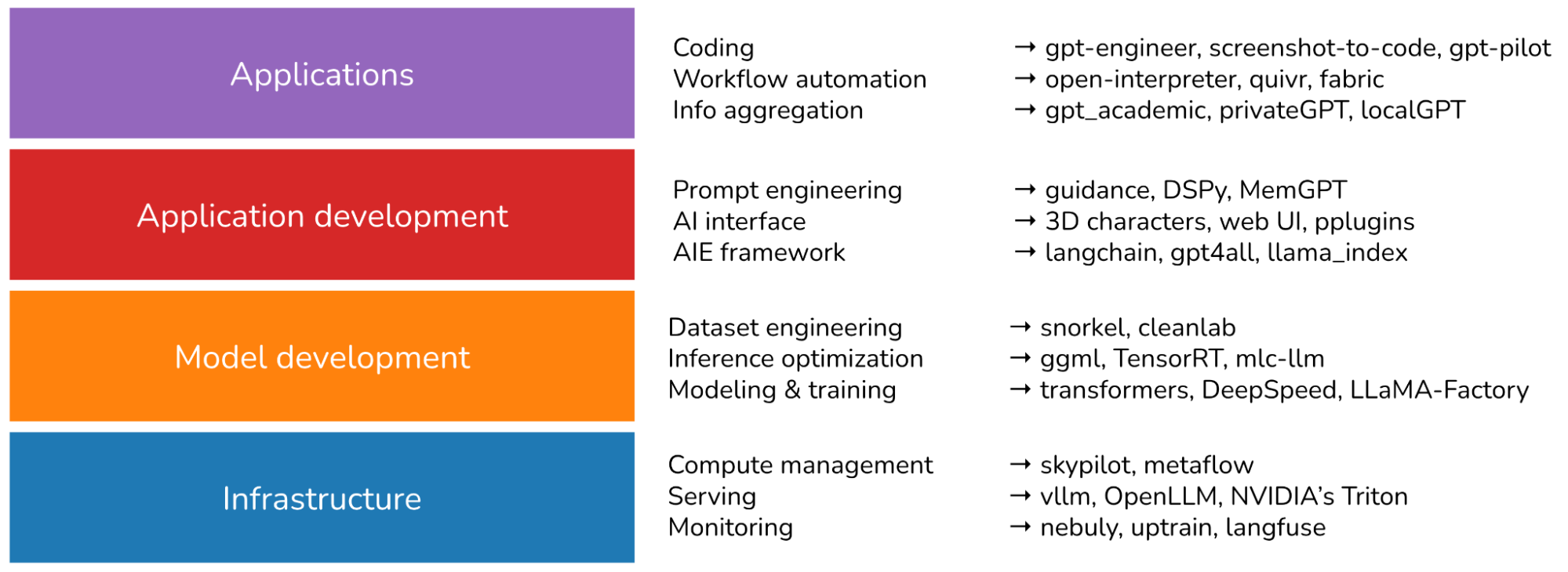
Infrastructure
At the bottom is the stack is infrastructure, which includes toolings for serving (vllm, NVIDIA’s Triton), compute management (skypilot), vector search and database (faiss, milvus, qdrant, lancedb), ….
Model development
This layer provides toolings for developing models, including frameworks for modeling & training (transformers, pytorch, DeepSpeed), inference optimization (ggml, openai/triton), dataset engineering, evaluation, ….. Anything that involves changing a model’s weights happens in this layer, including finetuning.
Application development With readily available models, anyone can develop applications on top of them. This is the layer that has seen the most actions in the last 2 years and is still rapidly evolving. This layer is also known as AI engineering.
Application development involves prompt engineering, RAG, AI interface, …
Outside of these 3 layers, I also have two other categories:
CompVis/stable-diffusion, openai/whisper, and facebookresearch/llama.Note: In an older version of this post, Applications was included as another layer in the stack.
I plotted the cumulative number of repos in each category month-over-month. There was an explosion of new toolings in 2023, after the introduction of Stable Diffusion and ChatGPT. The curve seems to flatten in September 2023 because of three potential reasons.
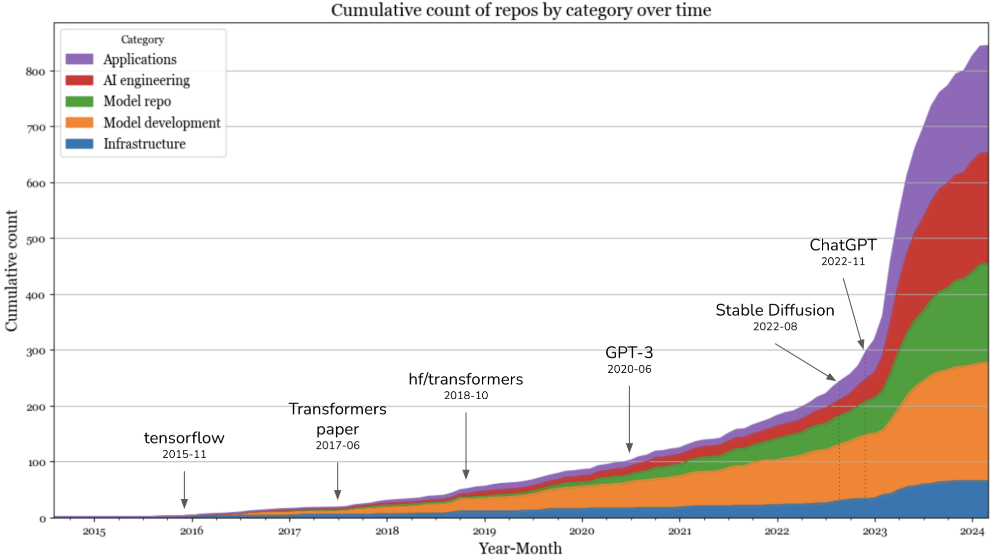
In 2023, the layers that saw the highest increases were the applications and application development layers. The infrastructure layer saw a little bit of growth, but it was far from the level of growth seen in other layers.
Not surprisingly, the most popular types of applications are coding, bots (e.g. role-playing, WhatsApp bots, Slack bots), and information aggregation (e.g. “let’s connect this to our Slack and ask it to summarize the messages each day”).
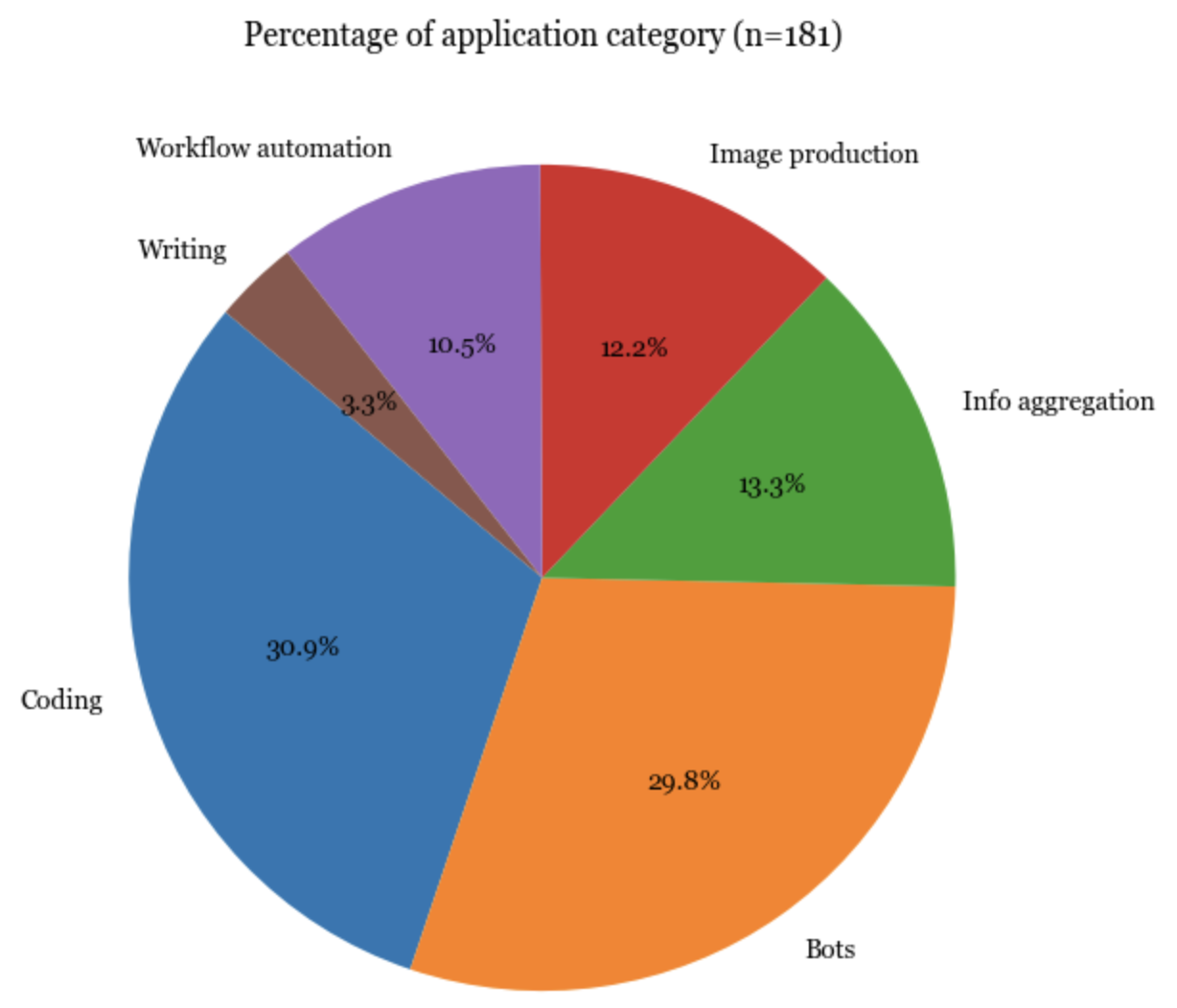
2023 was the year of AI engineering. Since many of them are similar, it’s hard to categorize the tools. I currently put them into the following categories: prompt engineering, AI interface, Agent, and AI engineering (AIE) framework.
Prompt engineering goes way beyond fiddling with prompts to cover things like constrained sampling (structured outputs), long-term memory management, prompt testing & evaluation, etc.
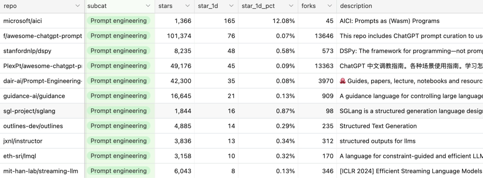
AI interface provides an interface for your end users to interact with your AI application. This is the category I’m the most excited about. Some of the interfaces that are gaining popularity are:
AIE framework is a catch-all term for all platforms that help you develop AI applications. Many of them are built around RAG, but many also provide other toolings such as monitoring, evaluation, etc.
Agent is a weird category, as many agent toolings are just sophisticated prompt engineering with potentially constrained generation (e.g. the model can only output the predetermined action) and plugin integration (e.g. to let the agent use tools).
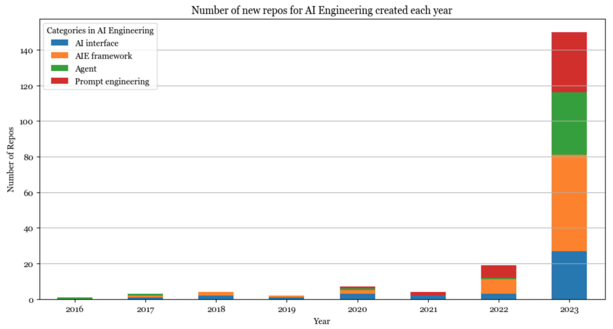
Pre-ChatGPT, the AI stack was dominated by model development. Model development’s biggest growth in 2023 came from increasing interest in inference optimization, evaluation, and parameter-efficient finetuning (which is grouped under Modeling & training).
Inference optimization has always been important, but the scale of foundation models today makes it crucial for latency and cost. The core approaches for optimization remain the same (quantization, low-ranked factorization, pruning, distillation), but many new techniques have been developed especially for the transformer architecture and the new generation of hardware. For example, in 2020, 16-bit quantization was considered state-of-the-art. Today, we’re seeing 2-bit quantization and even lower than 2-bit.
Similarly, evaluation has always been essential, but with many people today treating models as blackboxes, evaluation has become even more so. There are many new evaluation benchmarks and evaluation methods, such as comparative evaluation (see Chatbot Arena) and AI-as-a-judge.
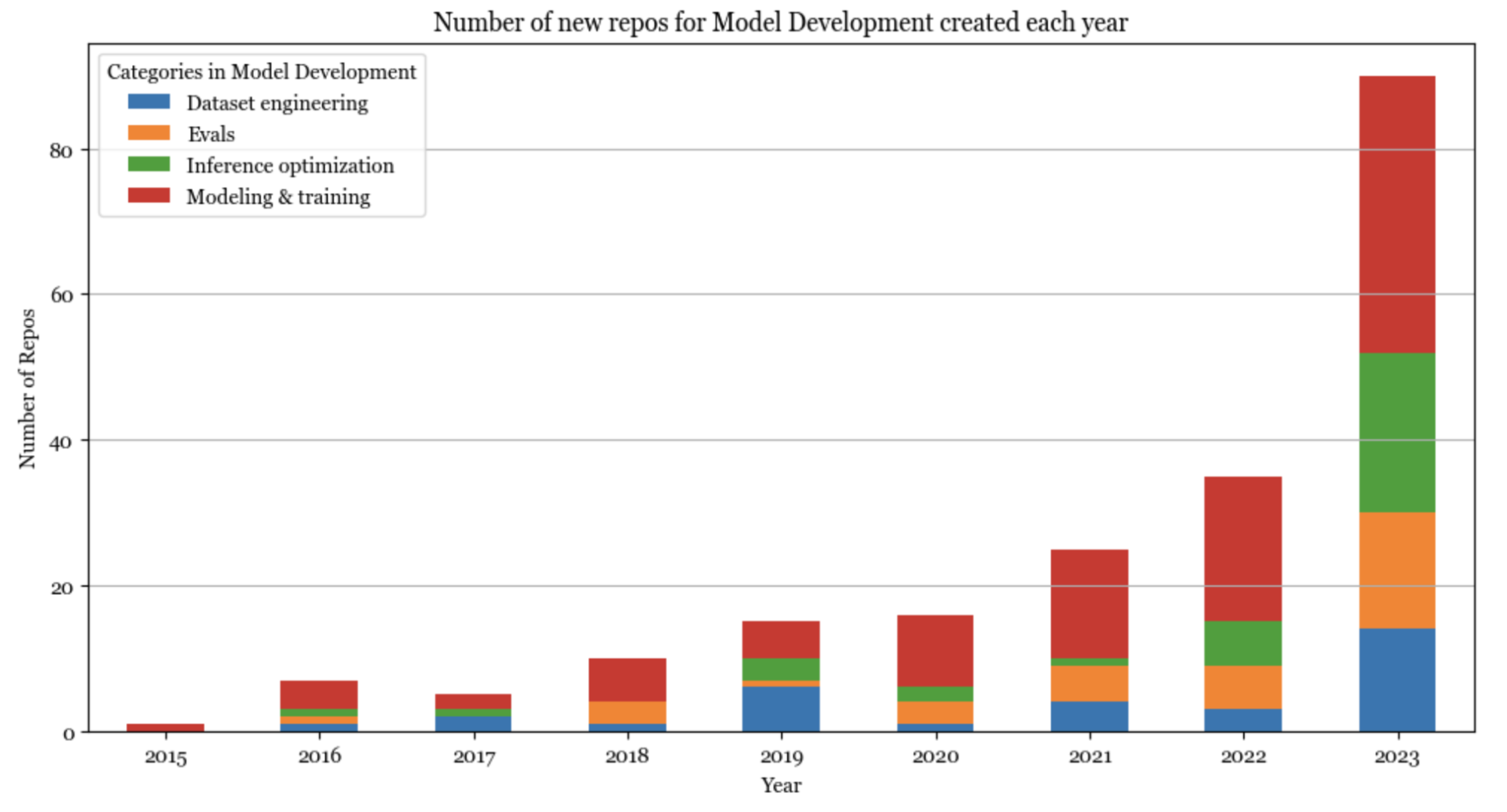
Infrastructure is about managing data, compute, and toolings for serving, monitoring, and other platform work. Despite all the changes that generative AI brought, the open source AI infrastructure layer remained more or less the same. This could also be because infrastructure products are typically not open sourced.
The newest category in this layer is vector database with companies like Qdrant, Pinecone, and LanceDB. However, many argue this shouldn’t be a category at all. Vector search has been around for a long time. Instead of building new databases just for vector search, existing database companies like DataStax and Redis are bringing vector search into where the data already is.
Open source software, like many things, follows the long tail distribution. A handful of accounts control a large portion of the repos.
845 repos are hosted on 594 unique GitHub accounts. There are 20 accounts with at least 4 repos. These top 20 accounts host 195 of the repos, or 23% of all the repos on the list. These 195 repos have gained a total of 1,650,000 stars.
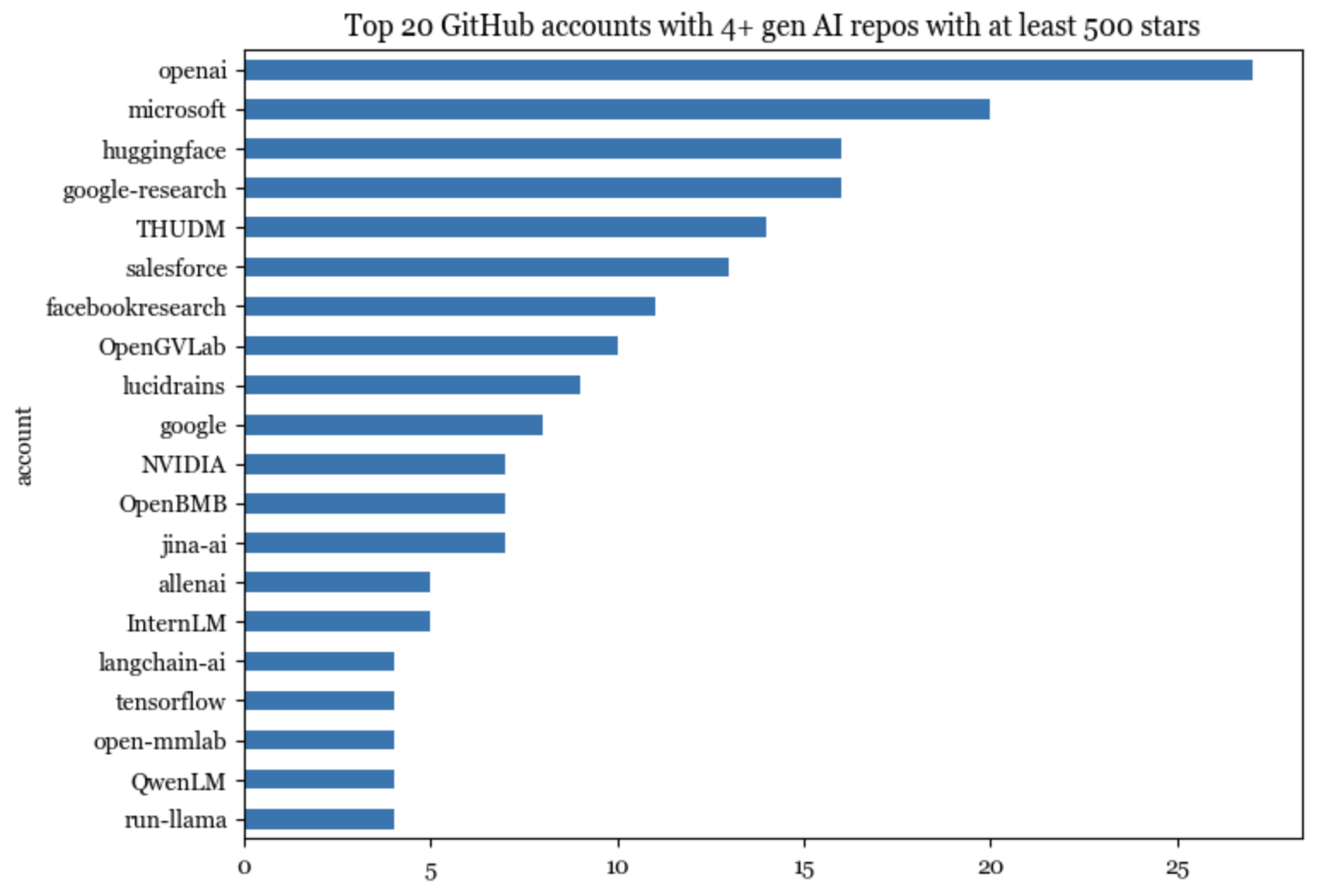
On Github, an account can be either an organization or an individual. 19/20 of the top accounts are organizations. Of those, 3 belong to Google: google-research, google, tensorflow.
The only individual account in these top 20 accounts is lucidrains. Among the top 20 accounts with the most number of stars (counting only gen AI repos), 4 are individual accounts:
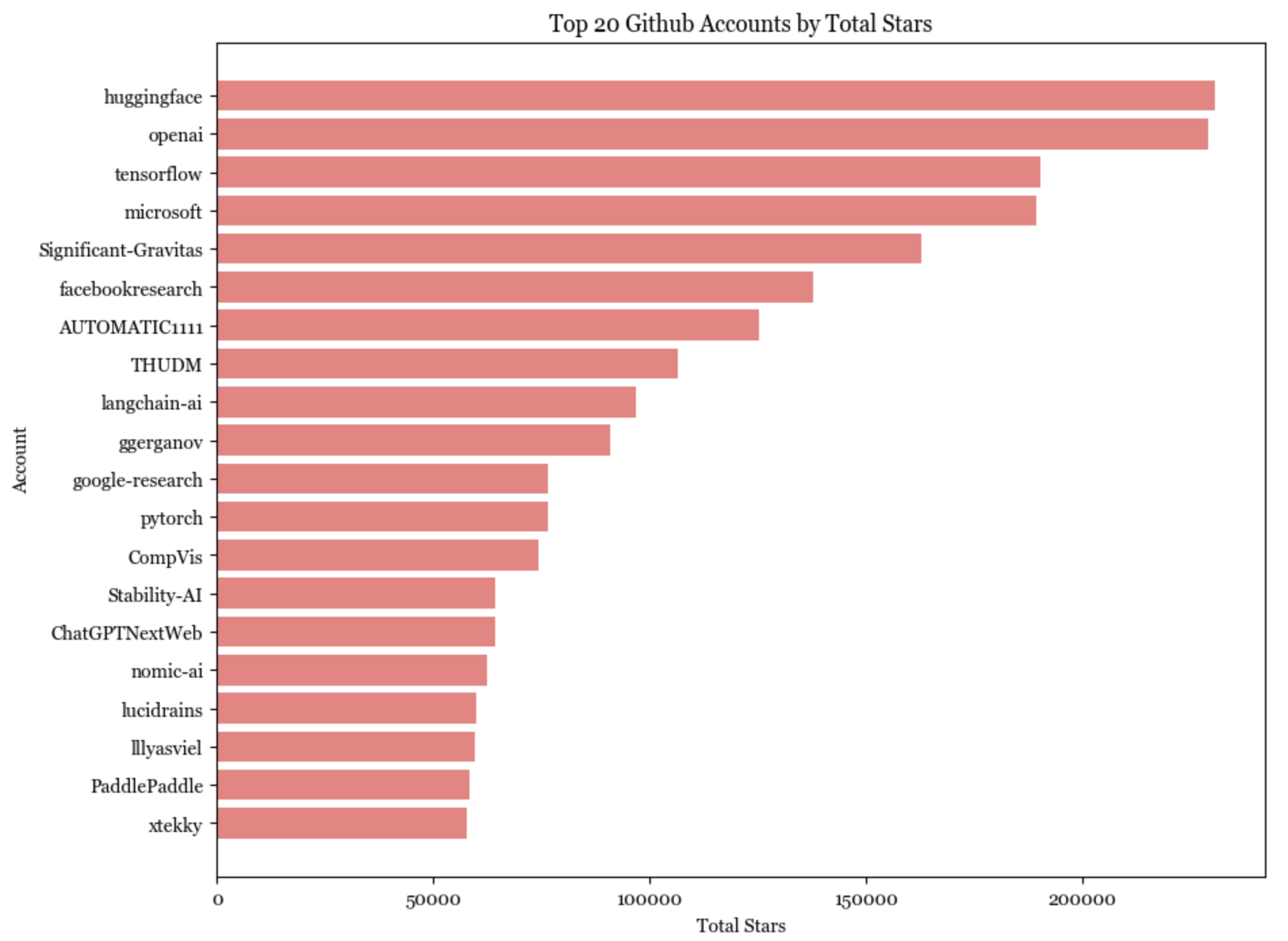
Unsurprisingly, the lower we go in the stack, the harder it is for individuals to build. Software in the infrastructure layer is the least likely to be started and hosted by individual accounts, whereas more than half of the applications are hosted by individuals.
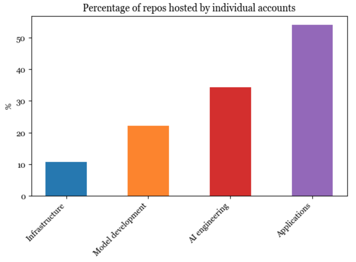
Applications started by individuals, on average, have gained more stars than applications started by organizations. Several people have speculated that we’ll see many very valuable one-person companies (see Sam Altman’s interview and Reddit discussion). I think they might be right.
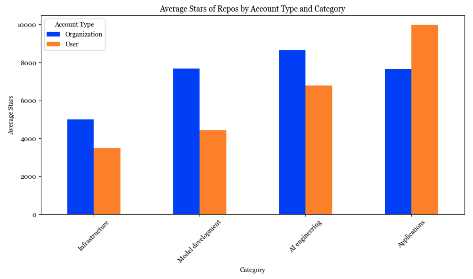
Over 20,000 developers have contributed to these 845 repos. In total, they’ve made almost a million contributions!
Among them, the 50 most active developers have made over 100,000 commits, averaging over 2,000 commits each. See the full list of the top 50 most active open source developers here.
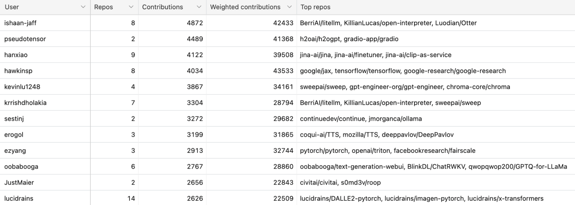
It’s been known for a long time that China’s AI ecosystem has diverged from the US (I also mentioned that in a 2020 blog post). At that time, I was under the impression that GitHub wasn’t widely used in China, and my view back then was perhaps colored by China’s 2013 ban on GitHub.
However, this impression is no longer true. There are many, many popular AI repos on GitHub targeting Chinese audiences, such that their descriptions are written in Chinese. There are repos for models developed for Chinese or Chinese + English, such as Qwen, ChatGLM3, Chinese-LLaMA.
While in the US, many research labs have moved away from the RNN architecture for language models, the RNN-based model family RWKV is still popular.
There are also AI engineering tools providing ways to integrate AI models into products popular in China like WeChat, QQ, DingTalk, etc. Many popular prompt engineering tools also have mirrors in Chinese.
Among the top 20 accounts on GitHub, 6 originated in China:
One pattern that I saw last year is that many repos quickly gained a massive amount of eyeballs, then quickly died down. Some of my friends call this the “hype curve”. Out of these 845 repos with at least 500 GitHub stars, 158 repos (18.8%) haven’t gained any new stars in the last 24 hours, and 37 repos (4.5%) haven’t gained any new stars in the last week.
Here are examples of the growth trajectory of two of such repos compared to the growth curve of two more sustained software. Even though these two examples shown here are no longer used, I think they were valuable in showing the community what was possible, and it was cool that the authors were able to get things out so fast.
So many cool ideas are being developed by the community. Here are some of my favorites.
Even though I included only 845 repos in my analysis, I went through several thousands of repos. I found this helpful for me to get a big-picture view of the seemingly overwhelming AI ecosystem. I hope the list is useful for you too. Please do let me know what repos I’m missing, and I’ll add them to the list!
2024-02-28 08:00:00
A challenge of building AI applications is choosing which model to use. What if we don’t have to? What if we can predict the best model for any prompt? Predictive human preference aims to predict which model users might prefer for a specific query.
Human preference has emerged to be both the Northstar and a powerful tool for AI model development. Human preference guides post-training techniques including RLHF and DPO. Human preference is also used to rank AI models, as used by LMSYS’s Chatbot Arena.
Chatbot Arena aims to determine which model is generally preferred. I wanted to see if it’s possible to predict which model is preferred for each query.
One use case of predictive human preference is model routing. For example, if we know in advance that for a prompt, users will prefer Claude Instant’s response over GPT-4, and Claude Instant is cheaper/faster than GPT-4, we can route this prompt to Claude Instant. Model routing has the potential to increase response quality while reducing costs and latency.
Another use case of predictive human preference is interpretability. Mapping out a model’s performance on different prompts can help us understand this model’s strengths and weaknesses. See section Experiment results for examples.
Here’s what predictive human preference for different model pairs looks like for the prompt “What’s the best way to cluster text embeddings?”. The predictions were generated by my toy preference predictor. The bright yellow color for the (GPT-4, GPT-3.5-Turbo) cell means that my predictor thinks GPT-4’s response is very likely to be preferred to that of GPT-3.5-Turbo’s for this prompt.
This post first discusses the correctness of Chatbot Arena, which will then be used as a baseline to evaluate the correctness of preference predictions. It then discusses how to build a preference predictor and the initial results.
Using preferential signals (comparisons) to rank models has grown in popularity in the last few years. Other than powering LMSYS’s Chatbot Arena, it’s also used by many model providers (Anthropic, Gemini, ChatGPT, etc.) to evaluate their models in production.
Side note: Friends who have deployed this in production told me that most users don’t read both options and just randomly vote for one. This introduces a lot of noise. However, the signals from the small percentage of users who vote correctly can sometimes be sufficient to help determine which model is preferred, as long as there’s minimal bias in the random voting.
Preferential ranking works in two steps:
For each request, two or more models are selected to respond. An evaluator, which can be human or AI, picks the winner. The evaluator shouldn’t know which models are being judged. Each comparison is called a match. This process results in a series of comparisons.
| Match ID | Prompt | Model A | Model B | Winner |
| 1 | … | Model 1 | Model 2 | Model 1 |
| 2 | … | Model 3 | Model 1 | Model 1 |
| 3 | … | Model 1 | Model 4 | Model 4 |
| ... | ... | ... | ... | ... |
From these comparisons, we need to compute the rankings of all models. The two most common ranking algorithms are Elo (from chess) and TrueSkill (from video games).
While Chatbot Arena refers to their model scores “Elo scores”, they actually don’t use Elo. In December 2023, they switched to Bradley-Terry but scaled the resulting scores to make them look Elo-like (see their notebook).
Given a history of match outcomes, the Bradley-Terry algorithm finds the model scores that maximize the likelihood of these match outcomes, turning model scoring into a maximum likelihood estimation problem. The input, for each training example, is the models that participate in the match. The output is the outcome of the match. Assuming there’s no draw, the outcome of a match is either 0 (a wins) or 1 (b wins).
Given the same match outcomes, different ranking algorithms can produce different rankings. For example, the ranking computed by Elo might differ from the ranking computed by Bradley-Terry. How do we know that a ranking is correct?
At its core, model ranking is a predictive problem. We compute a ranking from historical match outcomes and use it to predict future match outcomes. The quality of a ranking is determined by how accurately it can predict future match outcomes.
Let’s say we have a match between model A and model B. If model A has a higher score, meaning that the ranking algorithm predicts that A wins. If users indeed prefer the higher-ranking model, the ranking algorithm makes a correct prediction.
To compute the accuracy of Chatbot Arena ranking, I used their data published in July 2023, which consists of 33K crowd-sourced comparisons for matches among 20 models. I used this smaller dataset instead of their Jan 2024 dataset because this smaller dataset contains the prompt used for each match, which I need for predictive human preference. Benchmarking on this dataset allows me to compare my model with the Bradley-Terry algorithm later on.
Here’s an example from their July 2023 dataset.
| prompt | model_a | model_b | winner | model_a's response | model_b's response |
| who was the last monarch of uk | koala-13b | vicuna-13b | model_a | The last monarch of the United Kingdom was Queen Elizabeth II, who reigned from 1952 to 2020. | The current monarch of the United Kingdom is Queen Elizabeth II. She has been the monarch since 1952, and is the longest-reigning monarch in British history. |
For reference, the Bradley-Terry (BT) scores of the top 7 models in this dataset are as follows.
To create a test set, I randomly select 10% of the data (3300 examples). Each match has three possible outcomes: model_a wins, model_b wins, or tie. This can still be framed as a binary classification problem if we treat a tied match as two matches: one in which model_a wins and one in which model_b wins.
I found that for all non-tie matches in my test set, the model with the higher Bradley-Terry score is preferred 74.1% of the time. This means that if we always predict the higher-ranked model as the winner for a match, we’d have an accuracy of 74.1%.
| Test data | Output classes | # samples | BT's accuracy |
| All matches |
|
3,300 | 53.33% |
| Non-tie matches |
|
2,367 | 74.1% |
| Non-tie matches involving GPT-4 |
|
355 | 85.1% (always pick GPT-4 as winner) |
Back in July 2023, GPT-4 was considered the strongest model by a long shot (this was before Gemini, Mistral, Claude-v2). Did users always prefer GPT-4 to all other models? They didn’t. In 355 non-tie matches involving GPT-4, GPT-4 wins 85.1%.
This means that even though GPT-4 is the best model overall, there are prompts for which other models can outperform GPT-4. If we can figure out which prompts these are, and which models work best for them, we can route these prompts to the best-performing models, improving the response quality.
If a ranking algorithm is about figuring out which model is better overall, predictive human preference is about figuring out which model is better for each prompt. If we know in advance that for a particular prompt, GPT-3.5 works just as well as GPT-4, and GPT-3.5 is cheaper, we can route that prompt to GPT-3.5 instead. Or if we know that Mistral-7B works just as well as GPT-4 and Mistral-7B is faster, we can route our query to Mistral-7B instead.
Model routing can also help with budget planning. Say, you only have enough budget to serve 50% of queries on the strongest model, and the rest to a weaker model, you want to make sure that you send to the weaker model only the queries that you’re confident it can do well on.
I treat predictive human preference as a binary classification task. Given a match between 2 models, predict which one wins. If the probability of model_a winning is around 0.5, it can be considered a tie. If a Bradley-Terry model takes only (model_a, model_b) as the input, a preference predictor takes (prompt, model_a, model_b) as the input.

The architecture of my preference predictor looks like this. The model encoder and preference predictor are neural networks that can be trained independently or together. I used DistilBERT as my prompt encoder.

To train my model, I used 90% of LMSYS’s July 2023 dataset. I found that the predictor performed better using only non-tie matches (as opposed to using both tie and non-tie matches). I randomly flipped the order of models in a match 50% of the time.
To evaluate my model, I used 10% of this data. This is the same test data used to evaluate the correctness of Chatbot Arena’s ranking above.
| Split | All matches | Non-tie matches |
| Train | 29,700 | 20,927 |
| Test | 3,300 | 2,367 |
Note: I should’ve made a separate validation set for hyperparameter tuning. However, given that I didn’t have a lot of data and this is only a proof of concept, I didn’t do it. (I’m also lazy.) The matches are among 20 models, corresponding to 190 model pairs. 20,927 comparisons mean that, on average, there are only 110 comparisons per model pair.
I evaluated my preference predictor under two settings:
model_a and model_b as the input. This is to see whether this predictor, using only model names, can make better predictions about match outcomes than Chatbot Arena scores.(prompt, model_a, model_b) as the input. This is to see whether including prompts helps improve match outcome prediction.I found that for all non-tie matches, my preference predictor can predict the match outcome accurately 75% of the time if not using prompts, and 76.2% of the time if using prompts. This suggests that human preference for models does change depending on the prompt. While the improvement doesn’t seem much, a 2.1% improvement can be significant at scale.
| Eval data | # eval samples | Chatbot Arena |
Preference predictor (without prompts) |
Preference predictor (with prompts) |
| Non-tie matches | 2,367 | 74.1% | 75% | 76.2% |
| Non-tie matches involving GPT-4 | 355 | 85.1% | 86.2% | 87% |
Keep in mind that this predictor was trained with a small amount of crowd-sourced (e.g. noisy) data. The prompts crowdsourced are also simple. Among 33K prompts, 180 (0.55%) of them are “hello” and “hi”. These simple prompts are insufficient to distinguish strong models from weak ones. I suspect that with more/better data, the performance of this predictor can significantly improve.
Recall that 20 models correspond to 190 model pairs. To visualize how the predictor captures human preference, for each evaluation prompt, I generated 190 different inputs, one for each model pair.
I then visualized the 190 predictions for 190 model pairs in a 20 x 20 grid, as shown below for the prompt “Derive the elastic wave equation.” I only included 9 models in the plot to make it readable. The diagonal values refer to comparing a model to itself, so the predicted preference should be 0.5.
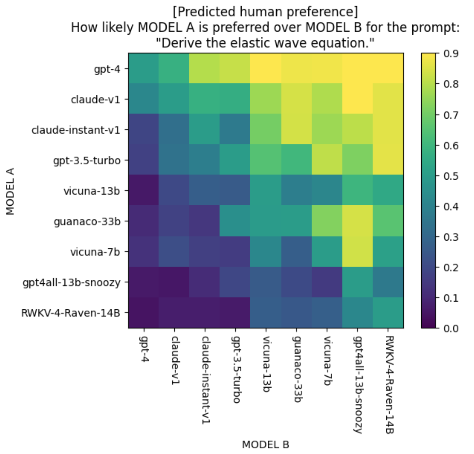
Given the predicted preference for all model pairs for a prompt, I used a Bradley-Terry model (the same ranking algorithm that LMSYS uses) to create a leaderboard for this prompt. I used the same scaling that LMSYS uses to make the scores look Elo-like. Here’s the ranking of the 9 models shown above for the query “Derive the elastic wave equation.”
This also means that with this preference predictor, we can create a leaderboard for any arbitrary subset of data. We can have a leaderboard specific to any domain.
|
|
|
| gpt-4 | 1214 |
| claude-v1 | 1162 |
| gpt-3.5-turbo | 1104 |
| claude-instant-v1 | 1110 |
| guanaco-33b | 1023 |
| vicuna-13b | 1007 |
| vicuna-7b | 985 |
| RWKV-4-Raven-14B | 970 |
| gpt4all-13b-snoozy | 915 |
Despite being a toy predictor, the model seems to be able to capture different models’ performance patterns. One pattern is that for simple prompts, weak models can do (nearly) as well as strong models. For more challenging prompts, however, users are much more likely to prefer stronger models. Here’s a visualization of predicted human preference for an easy prompt (“hello, how are you?”) and a challenging prompt (“Explain why Planc length …”).
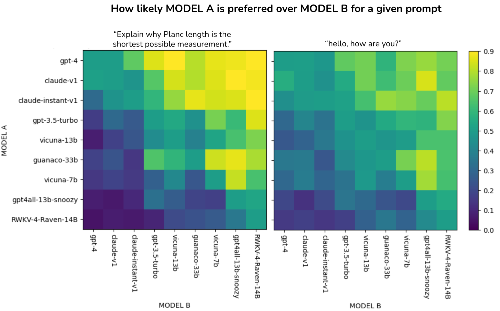
Here are the model rankings for these two prompts. The score spread for the simple prompt is much less than the score spread for the challenging prompt. The models that are ranked differently for these two prompts are highlighted in red.
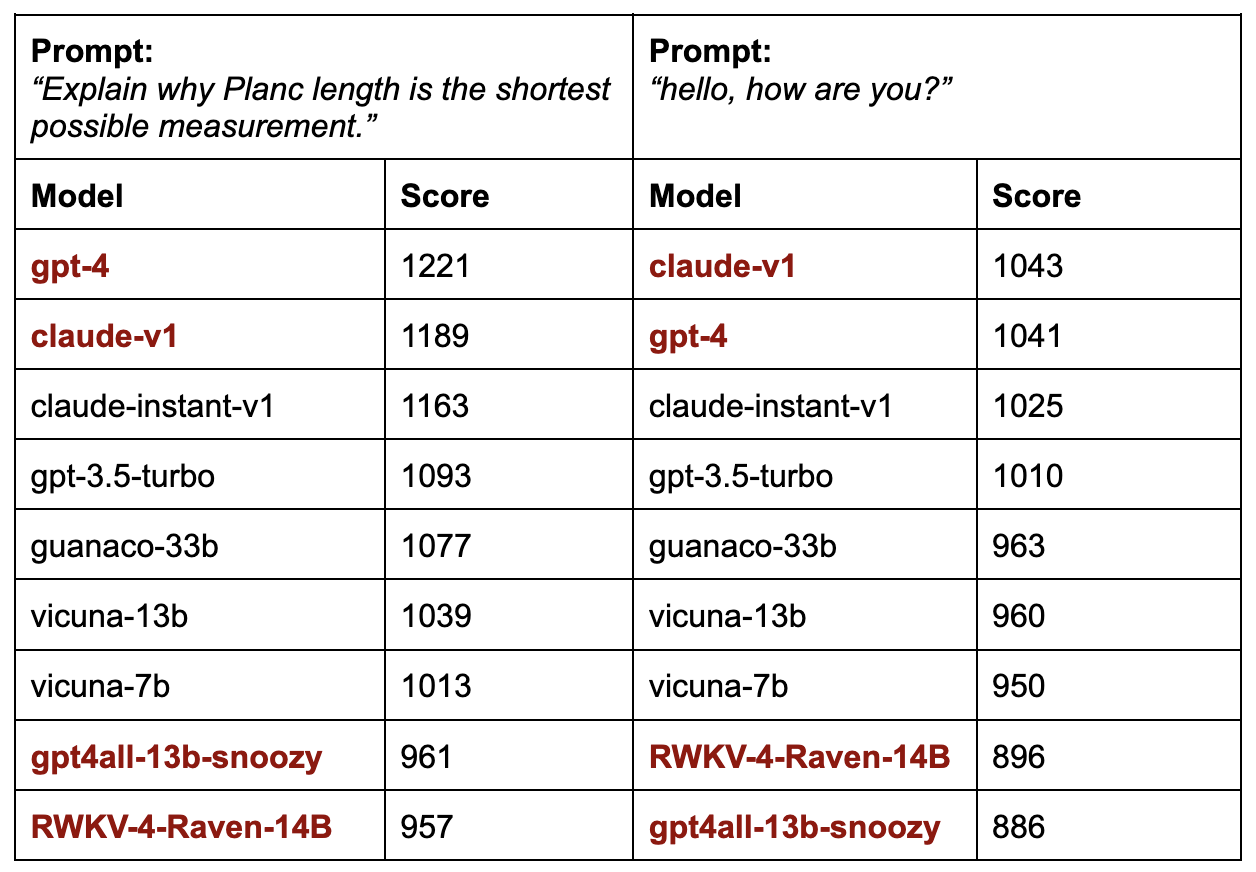
The predictor is also the most confident that GPT-4 will be preferred for queries in Russian and queries that involve code writing. For example, the average predicted win rate for the following Russian query of GPT-4 against all other models is 91.55%. Notice that for this query, while claude-v1 is predicted to do well on this query, claude-instant-v1 is predicted to do poorly.
My primitive experiment suggests that predictive human preference is feasible using a surprisingly small amount of data. There are many potential use cases for predictive human preference – model routing and interpretability are just two of them.
Predictive human reference is the first and the most important step in model routing (the other key step is routing strategy). With more and more models being developed, each with different capabilities and a cost structure, model routing has clear economic values.
I’m aware of four groups (two in stealth) that are working on model routing. One startup is Martian, which announced its $9M seed round. LMSYS is also working on model routing, which I think is a natural progression from their work in comparative evaluation.
While my experiment used human-annotated comparisons, LMSYS folks told me that due to the noisiness of crowd-sourced annotations and the costs of expert annotations, they’ve found that using GPT-4 to compare two responses works better. Depending on the complexity of the queries, generating 10,000 comparisons using GPT-4 would cost only $200 - 500, making this very affordable for companies that want to test it out.
This is the most fun side project I’ve worked on in a while, so I’d love to talk more about it. For those interested, I’ll be hosting a casual 30-minute discussion on predictive human preference on Tuesday, Mar 5, 9.30am PST. Join our Discord or email me if you want an invite!
Thanks Luke Metz for helping me with the experiments and coercing me into using JAX. While JAX is super cool and makes a lot of things easy, it also caused some of the weirdest bugs I’ve ever seen. I’m glad I used it though. Thanks Han-chung Lee for feedback on the plots.