2025-04-20 08:00:00
I just submitted another paper to SOSP 2025, and it’s hard to believe it’s been nearly four years since I started my PhD. A lot has changed since my last post about my PhD journey—looking back, I seemed pretty desperate then.
So here I am, reflecting on the past few years. I feel far more confident now—not just in my research decisions but in navigating the space of SysML in general.
When I started, I wasn’t sure about pretty much anything. But one thing I was certain about was ML inference. Admittedly, I didn’t grasp its full complexity or what compelling research directions existed, if at all. But I remembered reading in INFaaS that inference workloads account for 90% of ML infrastructure costs in AWS. That fact alone gave me hope—if inference drives such high traffic, it must be, or will become, important in the future.
Yet I kept wondering: Is there anything I can do at the model level? Many systems ML papers treated models as fixed-sized black boxes with deterministic execution latency and resource consumption. This assumption felt limiting.
That period was rough. Tons of methods for dynamic DNNs had already been proposed—early exit strategies, Mixture of Experts (MoE), model ensembles—but there just wasn’t a clear justification for designing systems specifically to optimize these approaches.
Honestly, I’m not sure how I made it through besides furiously searching ‘‘dynamic neural network’’, hoping to find something worth pursuing. Of course, the rise of ChatGPT changed everything, but that’s another story.
Everything shifted after my first paper was accepted to EMNLP. That was the moment I realized publishing isn’t as impossible as it seemed. Before, I kept trying to build an end-to-end system, a process that consumed far too much time.
Instead, I learned that starting with a clear motivation and simply writing it down first is a much better approach. Writing helps untangle confusion—it forces clarity.
The next few projects moved at a much faster pace. What changed? Honestly, the biggest shift was that I stopped fixating on the future. The long-term uncertainty used to kill my productivity—it felt overwhelming. But I realized that instead of worrying about whether a proposed method might fail, it’s far more productive to just write the next paragraph in Overleaf and move forward. After, if you write a paper, there exists a conference that is willing to accept it.
I’ll stop here and revisit this topic once I fully recover from the SOSP grind. For now, time to rest.
2024-09-01 08:00:00
TLDR; the Stichable Neural Networks paper includes some interesting concepts. It allows the creation of multiple neural networks with varying complexity and performance trade-offs from a family of pretrained models.
A key question about combining sub-networks from different pretrained models is how to maintain accuracy. The paper concludes that the final performance of these combinations is nearly predictable due to an interpolation-like performance curve between anchors. This predictability allows for selective pre-training of stitches based on various deployment scenarios.
Anchors that are pretrained on different tasks can learn very different representations due to the large distribution gap of different domains. Therefore, the selected anchors should be consistent in terms of the pretrained domain.
SN-Net is built upon pretrained models. Therefore, the anchors have already learned good representations, which allows to directly obtain an accurate transformation matrix by solving the least squares problem:
$$||AM_o - B|| = min||AM - b||_F$$
where $A \in R^{N \times D_1}$ and \(B \in R^{N \times D_2}\) are two feature maps of the same spatial size but with different number of hidden dimensions.
This function indicates a closed form expression based on singular value decomposition, in which case the optimal solution can be achieved through an orthogonal projection in the space of matrices:
$$M_o = A^\dagger B$$
where $A^\dagger$ denotes the Moore-Penrose pseudoinverse of $A$.
SN-Net takes Fast-to-Slow as the default stitching direction, meaning it will stitch bigger and slower network after smaller and faster networks to achieve better model performance. Besides, it also proposes a nearest stitching strategy by limiting the stitching between two anchors of the nearest model complexity/performance.
Prior works shows neighboring layers dealing with the same scale feature maps share similar representations. Therefore, SN-Net uses slideing window: where the same window shares a common stitching layer.
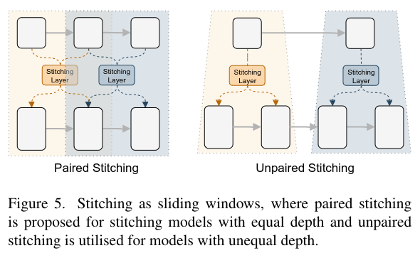
The stitching space is controlled by the configuring the sliding window kernel size $k$ and step size $s$.
The training algorithm of SN-Net can be described as:
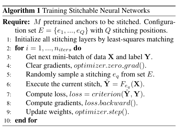
The training algorithm can be summarized as:
2024-08-28 08:00:00
This is an archive including blogs I find useful or interesting. Hopefully the updates will keep coming.
2022-08-30 08:00:00
In the previous post, we’ve explored how to write primitive functions in TensorIR. Here, we will see how to transform TensorIR into other (potentially more performant) variants. The content is drived from the mlc course taught by Tianqi Chen.
A batched matrix multiplication followed by a ReLu operation can be expressed using numpy as:
def lnumpy_mm_relu_v2(A: np.ndarray, B: np.ndarray, C: np.ndarray):
 Y = np.empty((16, 128, 128), dtype="float32")
 for n in range(16):
 for i in range(128):
 for j in range(128):
 for k in range(128):
 if k == 0:
 Y[n, i, j] = 0
 Y[n, i, j] = Y[n, i, j] + A[n, i, k] * B[n, k, j]
 for n in range(16):
 for i in range(128):
 for j in range(128):
 C[n, i, j] = max(Y[n, i, j], 0)
Translating the numpy code into TensorIR we get:
@tvm.script.ir_module
class MyBmmRule:
 @T.prim_func
 def bmm_relu(A: T.Buffer[(16, 128, 128), "float32"],
 W: T.Buffer[(16, 128, 128), "float32"],
 Y: T.Buffer[(16, 128, 128), "float32"]):
 T.func_attr({"global_symbol": "bmm_relu", "tir.noalias": True})
 # we must to allocate the buffer here!
 Y_ = T.alloc_buffer([16, 128, 128], dtype="float32")
 for n, i, j, k in T.grid(16, 128, 128, 128):
 with T.block("M"):
 vn = T.axis.spatial(16, n)
 vi = T.axis.spatial(128, i)
 vj = T.axis.spatial(128, j)
 vk = T.axis.reduce(128, k)
 with T.init():
 Y_[vn, vi, vj] = T.float32(0)
 Y_[vn, vi, vj] += A[vn, vi, vk] * W[vn, vk, vj]
 for n, i, j in T.grid(16, 128, 128):
 with T.block("R"):
 vn = T.axis.spatial(16, n)
 vi = T.axis.spatial(128, i)
 vj = T.axis.spatial(128, j)
 Y[vn, vi, vj] = T.max(Y_[vn, vi, vj], T.float32(0))
Our ultimate goal is to transform the TensorIR above to the following form:
@tvm.script.ir_module
class TargetModule:
 @T.prim_func
 def bmm_relu(A: T.Buffer[(16, 128, 128), "float32"], B: T.Buffer[(16, 128, 128), "float32"], C: T.Buffer[(16, 128, 128), "float32"]) -> None:
 T.func_attr({"global_symbol": "bmm_relu", "tir.noalias": True})
 Y = T.alloc_buffer([16, 128, 128], dtype="float32")
 for i0 in T.parallel(16):
 for i1, i2_0 in T.grid(128, 16):
 for ax0_init in T.vectorized(8):
 with T.block("M_init"):
 n, i = T.axis.remap("SS", [i0, i1])
 j = T.axis.spatial(128, i2_0 * 8 + ax0_init)
 Y[n, i, j] = T.float32(0)
 for ax1_0 in T.serial(32):
 for ax1_1 in T.unroll(4):
 for ax0 in T.serial(8):
 with T.block("M_update"):
 n, i = T.axis.remap("SS", [i0, i1])
 j = T.axis.spatial(128, i2_0 * 8 + ax0)
 k = T.axis.reduce(128, ax1_0 * 4 + ax1_1)
 Y[n, i, j] = Y[n, i, j] + A[n, i, k] * B[n, k, j]
 for i2_1 in T.vectorized(8):
 with T.block("R"):
 n, i = T.axis.remap("SS", [i0, i1])
 j = T.axis.spatial(128, i2_0 * 8 + i2_1)
 C[n, i, j] = T.max(Y[n, i, j], T.float32(0))
Before we perform the transformation, let’s understand what the transformed TensorIR is doing by looking at several loops here.
First, taking a look at
for i1, i2_0 in T.grid(128, 16):
 for ax0_init in T.vectorized(8):
 with T.block("M_init"):
 n, i = T.axis.remap("SS", [i0, i1])
 j = T.axis.spatial(128, i2_0 * 8 + ax0_init)
 Y[n, i, j] = T.float32(0)
The code block is initializing the Y matrix to be 0. But it does so by initializing every 8 consecutive elements in each row of Y using a vectorized operation (which might be faster).
The next loop is bit tricky:
for ax1_0 in T.serial(32):
 for ax1_1 in T.unroll(4):
 for ax0 in T.serial(8):
 with T.block("M_update"):
 n, i = T.axis.remap("SS", [i0, i1])
 j = T.axis.spatial(128, i2_0 * 8 + ax0)
 k = T.axis.reduce(128, ax1_0 * 4 + ax1_1)
 Y[n, i, j] = Y[n, i, j] + A[n, i, k] * B[n, k, j]
This loop is actually performing the matrix multiplication of A and B. We mutiply a row in A with a column in B and sum up the result into a number.
Here, i is mapped to i1, which means we access A one row at a time.i k = T.axis.reduce(128, ax1_0 * 4 + ax1_1) means we access one row in matrix A and one column in matrix B sequentially duing mutiplying, while applying unrolling in hope for better access efficency (\(128 = 32\times 4))). j = T.axis.spatial(128, i2_0 * 8 + ax0) really just means accessing each column sequentially, nothing special.
To perform tranformation on any TensorIP, it’s very important to follow the steps listed below:
Applying step 1, 2, and 3, we first get the block from the original TensorIR:
sch = tvm.tir.Schedule(MyBmmRule)
# Step 1. Get blocks
block_M = sch.get_block("M", func_name="bmm_relu")

# Step 2. Get loops
n, i, j, k = sch.get_loops(block_M)

# Step 3. Organize loops
k0, k1 = sch.split(k, factors=[32, 4])
j0, j1 = sch.split(j, factors=[16, 8])
The reason we split k and j in such a way is: we already mentioned k dimension is accessed sequentially but with unrolling (4) applied; when matrix Y is initialized, a vectorized operation (applied on 8 elements) is applied to dimension j, or every 8 elements in one row(TVM is row-major, therefore might be faster).
But the next question is: how do we reorder the spitted loop? I spent a lot of time trying to figure that out. Turns out the simplest way is to write out the implementation in numpy and proceed from there. Remember, we’ve already splitted k and j, which are used during matrix multiplication, so our new matrix multipliation in numy would be:
for j0 in range(16):
 for k0 in range(32):
 for k1 in range(4):
 for j1 in range(8):
 Y[i, 8*j0+j1] += A[i, 4*k0 + k1] * B[4*k0+k1, 8*j0+j1]
Because we move the the next column in B after traversing the previous column, we will put j1 at the innermost loop. Therefore, the transformation for TensorIR would be:
sch.reorder(j0, k0, k1, j1)
We can print out the transformed TensorIR with print(sch.mod.script()):
@tvm.script.ir_module
class Module:
 @tir.prim_func
 def bmm_relu(A: tir.Buffer[(16, 128, 128), "float32"], B: tir.Buffer[(16, 128, 128), "float32"], C: tir.Buffer[(16, 128, 128), "float32"]) -> None:
 tir.func_attr({"global_symbol": "bmm_relu", "tir.noalias": True})
 Y = tir.alloc_buffer([16, 128, 128], dtype="float32")
 for n in tir.parallel(16):
 for i, j_0, k_0, k_1, j_1 in tir.grid(128, 16, 32, 4, 8):
 with tir.block("M"):
 vn, vi = tir.axis.remap("SS", [n, i])
 vj = tir.axis.spatial(128, j_0 * 8 + j_1)
 vk = tir.axis.reduce(128, k_0 * 4 + k_1)
 tir.reads(A[vn, vi, vk], B[vn, vk, vj])
 tir.writes(Y[vn, vi, vj])
 with tir.init():
 Y[vn, vi, vj] = tir.float32(0)
 Y[vn, vi, vj] = Y[vn, vi, vj] + A[vn, vi, vk] * B[vn, vk, vj]
 for n, i, j in tir.grid(16, 128, 128):
 with tir.block("R"):
 vn, vi, vj = tir.axis.remap("SSS", [n, i, j])
 tir.reads(Y[vn, vi, vj])
 tir.writes(C[vn, vi, vj])
 C[vn, vi, vj] = tir.max(Y[vn, vi, vj], tir.float32(0))
Now, we just need to move the ReLu operation (for n, i, j in tir.grid(16, 128, 128):) into the loop above:
block_M = sch.get_block("M", func_name="bmm_relu")
sch.reverse_compute_at(block_M, j0)
Step 4 involves seperating initialization and matrix multiplication, therefore we use M_init = sch.decompose_reduction(block_M, k0), which results in:
@tvm.script.ir_module
class Module:
 @tir.prim_func
 def bmm_relu(A: tir.Buffer[(16, 128, 128), "float32"], B: tir.Buffer[(16, 128, 128), "float32"], C: tir.Buffer[(16, 128, 128), "float32"]) -> None:
 # function attr dict
 tir.func_attr({"global_symbol": "bmm_relu", "tir.noalias": True})
 # body
 # with tir.block("root")
 Y = tir.alloc_buffer([16, 128, 128], dtype="float32")
 for n in tir.parallel(16):
 for i, j_0 in tir.grid(128, 16):
 for j_1_init in tir.serial(8):
 with tir.block("M_init"):
 vn, vi = tir.axis.remap("SS", [n, i])
 vj = tir.axis.spatial(128, j_0 * 8 + j_1_init)
 tir.reads()
 tir.writes(Y[vn, vi, vj])
 Y[vn, vi, vj] = tir.float32(0)
 for k_0, k_1, j_1 in tir.grid(32, 4, 8):
 with tir.block("M_update"):
 vn, vi = tir.axis.remap("SS", [n, i])
 vj = tir.axis.spatial(128, j_0 * 8 + j_1)
 vk = tir.axis.reduce(128, k_0 * 4 + k_1)
 tir.reads(Y[vn, vi, vj], A[vn, vi, vk], B[vn, vk, vj])
 tir.writes(Y[vn, vi, vj])
 Y[vn, vi, vj] = Y[vn, vi, vj] + A[vn, vi, vk] * B[vn, vk, vj]
 for ax0 in tir.serial(8):
 with tir.block("R"):
 vn, vi = tir.axis.remap("SS", [n, i])
 vj = tir.axis.spatial(128, j_0 * 8 + ax0)
 tir.reads(Y[vn, vi, vj])
 tir.writes(C[vn, vi, vj])
 C[vn, vi, vj] = tir.max(Y[vn, vi, vj], tir.float32(0))
The final step is easy, just apply vectorize/parallel/unroll onto corresponding loop:
n, i, j_0, j_1_init = sch.get_loops(M_init)
sch.vectorize(j_1_init)

n, i, j_0, i2_1 = sch.get_loops(block_R)
sch.vectorize(i2_1)

block_M_update = sch.get_block("M_update", func_name="bmm_relu")
n, i, j_0, k_0, k_1, j_1 = sch.get_loops(block_M_update)
Print out the final TensorIR to find out its final form ( ͡❛ ͜ʖ ͡❛).
2022-08-28 08:00:00
TensorIR is a compiler abstraction for optimizing programs with tensor computation primitives in TVM. Imagine a DNN task as a graph, where each node represents a tensor computation. TensorIR explains how each node/tensor computation primitive in the graph is carried out. This post explains my attempt to implement 2D convolution using TensorIR. It is derived from the Machine Learning Compilation course offered by Tianqi Chen.
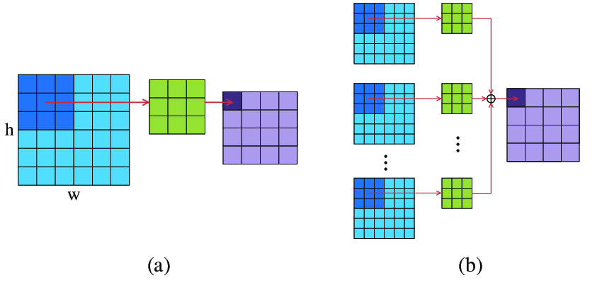
2D convolution is a common operation in image processing. The image below captures how 2D convolution operates. I won’t go into details here. But you can find plenty information online regarding convolution.
First, we initialize both the input matrix and the weight matrix:
# batch, input_channel_dim, image_height, image_width, output_channel_dim, kernel_width & height
N, CI, H, W, CO, K = 1, 1, 8, 8, 2, 3
# output_height, output_width, assuming kernel has stride=1 and padding=0
OUT_H, OUT_W = H - K + 1, W - K + 1
data = np.arange(N*CI*H*W).reshape(N, CI, H, W)
weight = np.arange(CO*CI*K*K).reshape(CO, CI, K, K)
We can validate the results using torch.nn.functional.conv2d() from PyTorch.
One thing Tianqi recommended for starters is to write the implementation first in numpy, and then translate the numpy implementation to TensorIR. I started my implementation directly from TensorIR, before totally getting confused. So here’s how I approach the problem.
First, and perhaps most importantly, you should figure out the accessing pattern of the output matrix, and gradually fill up the compute rules for each element in the output matrix. So, we know the output matrix has a shape of (N, CO, OUT_H, OUT_w) (which corresponds to batch, number of output channels, output height, and output width). The numpy loop will look like:
for b in np.arange(0, N):
 for co in np.arange(0, CO):
 for h in np.arange(0, OUT_H):
 for w in np.arange(0, OUT_W):
 Y[b, co, h, w] = 0
Here, we access element in the output matrix one by one and initialize each element to be 0. Next, we will try to figure out how to compute each element. We know each element in the output matrix is just the sum of element-wise multiplication of both the 2D convolutional kernel (1 by 3 by 3) and the corresponding area in the input matrix (1 by 3 by 3):
for b in np.arange(0, N):
 for co in np.arange(0, CO):
 for h in np.arange(0, OUT_H):
 for w in np.arange(0, OUT_W):
 # init to 0
 Y[b, co, h, w] = 0
 # 2d conv kernel
 for ci in np.arange(0, CI):
 for kh in np.arange(0, K):
 for kw in np.arange(0, K):
 # reduction
 Y[b, co, h, w] += A[b, ci, h+kh, w+kw] * W[co, ci, kh, kw]
We can verify the function has the same output as torch.nn.functional.conv2d() from PyTorch.
The next part is to translate the numpy code into TensorIR. I won’t go into every the details of every single line here, but you can find all explanations from this note.
The nested loop can be encapsulated using T.grid() like this:
@tvm.script.ir_module
class MyConv:
 @T.prim_func
 def conv2d(data: T.Buffer[(N, CI, H, W), "int64"],
 weight: T.Buffer[(CO, CI, K, K), "int64"],
 result: T.Buffer[(N, CO, OUT_H, OUT_W), "int64"]):
 T.func_attr({"global_symbol": "conv2d", "tir.noalias": True})
 # loop through each elem in the output matrix
 for b, o, h, w in T.grid(N, CO, OUT_H, OUT_W):
 # kernel access pattern
 for kc, kh, kw in T.grid(CI, K, K):
Next, we define the block (a basic unit of computation in TensorIR). A block contains a set of block axes (vi, vj, vk) and computations defined around them. Here, we define the property about each block axes:
class MyConv:
 @T.prim_func
 def conv2d(data: T.Buffer[(N, CI, H, W), "int64"],
 weight: T.Buffer[(CO, CI, K, K), "int64"],
 result: T.Buffer[(N, CO, OUT_H, OUT_W), "int64"]):
 T.func_attr({"global_symbol": "conv2d", "tir.noalias": True})
 # impl
 for b, o, h, w in T.grid(N, CO, OUT_H, OUT_W):
 for kc, kh, kw in T.grid(CI, K, K):
 with T.block("A"):
 vb = T.axis.spatial(N, b)
 vc_o = T.axis.spatial(CO, o)
 vh = T.axis.spatial(OUT_H, h)
 vw = T.axis.spatial(OUT_W, w)
 vc_i = T.axis.reduce(CI, kc)
 vw_h = T.axis.reduce(K, kh)
 vw_w = T.axis.reduce(K, kw)
The outer loop all receives T.axis.spatial(), because we access each element in the output matrix element by element (spatially), without doing anything else. On the other hand, we see parameters in the innter loop receives T.axis.reduce(). Remember, each element in the output matrix is just the sum of element-wise multiplication of both the 2D convolutional kernel (1 by 3 by 3) and the corresponding area in the input matrix (1 by 3 by 3). Therefore, after the element-wise multiplication finishes, we need perform a reduction operation over all three axes. More concretely, we will sum up all elements in the row(K), column(K), and channel(CI): (1, 3, 3) -> (1)
@tvm.script.ir_module
class MyConv:
 @T.prim_func
 def conv2d(data: T.Buffer[(N, CI, H, W), "int64"],
 weight: T.Buffer[(CO, CI, K, K), "int64"],
 result: T.Buffer[(N, CO, OUT_H, OUT_W), "int64"]):
 T.func_attr({"global_symbol": "conv2d", "tir.noalias": True})
 # impl
 for b, o, h, w in T.grid(N, CO, OUT_H, OUT_W):
 for kc, kh, kw in T.grid(CI, K, K):
 with T.block("A"):
 vb = T.axis.spatial(N, b)
 vc_o = T.axis.spatial(CO, o)
 vh = T.axis.spatial(OUT_H, h)
 vw = T.axis.spatial(OUT_W, w)
 vc_i = T.axis.reduce(CI, kc)
 vw_h = T.axis.reduce(K, kh)
 vw_w = T.axis.reduce(K, kw)

 with T.init():
 result[vb, vc_o, vh, vw] = T.int64(0)
 # compute rule
 result[vb, vc_o, vh, vw] += data[vb, vc_i, vh+vw_h, vw+vw_w] * weight[vc_o, vc_i, vw_h, vw_w]
2022-03-31 08:00:00
Google recently released the paper about its new ML system called Pathways. I’m a bit surprised since I expect it to introduce a brand new model architecture. In fact, this paper is not easy to digest at all. I feel like it’s written for people who spent many years developing ML frameworks. Anyway, we will try to understand why it is developed and how it works. Also, you should check this post (in Chinese). This post explains many concepts in Pathways much more clearly. Many contents here are credited to this post.
This paper spends a long time discussing single-controller and multi-controller. It’s really confusing to understand all these SPMD, MPMD, single-controller, and multi-controller stuffs. Pathways claims the future ML framework should go back to single-controller. By “back” I mean ML frameworks were originally single-controller, then they adopted multi-controller. Now, we are going back to single-controller again.
TensorFlow v1 is a classic example of single-controller system. The high level idea is the user would define a dataflow graph through a Python client. This graph is then submitted to the session.run (runtime system). The system consists of a single master and many other workers. The mater will compile and the dataflow graph submitted by the client, then divides the graph into sub-graphs. Then the master submits those subgraphs to other workers.
In this case, each worker computes its own share of sub-graph. The client + master are the controller.
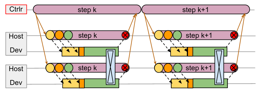
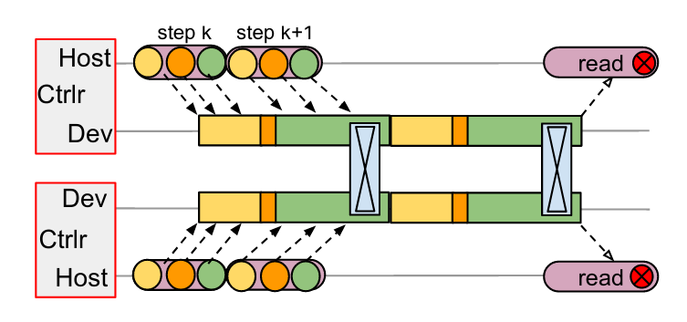
As the paper suggests, dispatching computations in a single-controller system requires communnication across (data center network) DCN. All the orange lines are control messages flowing through DCN. We can see the workers are idle for a long time between each step, even though there’s no gap between adjust steps on the controller.
The controller submits jobs to all workers in each step, then waits all workers to finish computing their own sub-graphs. The problem is: 1) waiting for all workers to finish computation in a lock-step fashion is inefficient; 2) send and wait for control messages (orange line) is costly since these messages go through slow DCN.
Contrary to single-controller systems, multi-controller systems like Jax adopts a different philosophy. Under multi-controller systems, each worker shares the same code and executes different stage/branch of the code. This is why they are called SPMD systems (single-program-multiple-data).
Take MPI process as an example, every MPI process is an entrance (client) to the program (In single-controller systems, only the client-master can be the entrance).
Since multi-controller systems doesn’t have a centralized coordinator, all workers in can initiate communication with each other, using much faster channels such as PCIe or NVLink. In the multi-controller graph, the black dotted lines represents message between hosts and devices (through PCIe); the communication between devices happens through fast NVLink. So we don’t have the big overhead introduced by DCN.
If you want to get a taste of how PyTorch vs TensorFlow v1’s (multi-controller vs single-controller) programming style feels like, here are two examples: Writing Distributed Applications with PyTorch and End-to-End Tutorial for Distributed TensorFlow 1.x.
We could stick with multi-controller systems forever. If every worker node shares symmetric workloads and communications (like all-reduce, all-gather, etc.), then there’s nothing to be worried about. After all, multi-controller seems much more efficient than single-controller based on what we’ve discussed so far.
However, pipeline parallelism changes the story. Under pipeline parallelism, different workers in the pipeline will execute at different programs. Thus we have MPMD (multi-program-multi-data). For example, we can have one worker doing convolution for batch 1 while another worker is doing encoding work on batch 2. At each stage of the pipeline, the worker is doing different jobs on a different data batch (think of a CPU pipeline where each stage is executing different instructions).
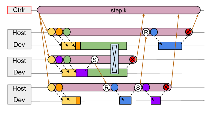
Take the above graph as an example, assume we have three workers 1, 2, 3 from top to bottom. Each worker is performing asymmetric workloads and doing irregular point-to-point communications (instead of symmetric communications like all-gather). Obviously, multi-controller doesn’t fit into this kind of workload. How do you write a single copy of code that does all these irregular communications under multi-process scenarios?
Thus, Pathways proposes we should go back to single-controller, so that we can let the master node handle all these nasty communication patterns.
Single-Controller brings back gang-scheduling and centralized coordinator. The reason to use gang-scheduling and centralized coordinator is to help preventing deadlocks. However, the rational behind this design decision is hard to interpret from reading the paper. I’m going to use the post from Jinhui Yan (the developer behind OneFlow) to explain why gang-scheduling and centralized coordinator prevent deadlocks.
Gang-scheduling is essential in the case of TPUs, since they are single-threaded and only run non-preemptible kernels, so the system will deadlock if communicating computations are not enqueued in a consistent order.
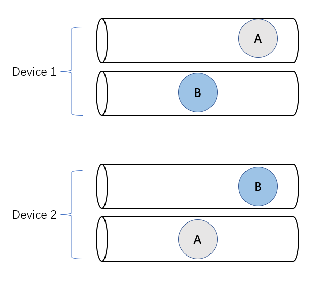
We can think of a computing device as a FIFO task queue (e,g. CUDA streams, TPU, or CPU…). Each FIFO task queue essentially have a stream of tasks to process.
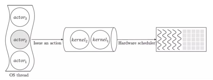
The paper emphasizes that TPUs are single-threaded and only run non-preemptible kernels. That means we can think of each TPU as a single FIFO task queue. Once we enqueue a task, it can not be preempted from the queue. We need to wait until this task finishes its computation before we can execute the next task in the queue. This is a problem!
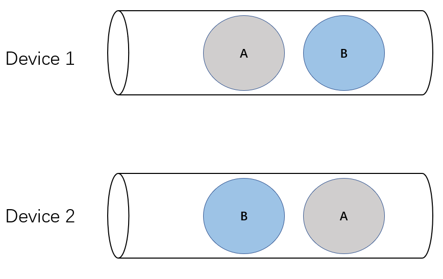
Imagine we have two devices (1 and 2), represented as two FIFO queues. Device 1 chooses to enqueue task A first and then B; device 2 decides to enqueue task B first and then A. Both tasks A and B are performing an all-scatter operation. Therefore, task A on device 1 needs to wait for messages from task A on device 2. Similarly, task B on device 2 needs to wait for messages from task B on device 1.
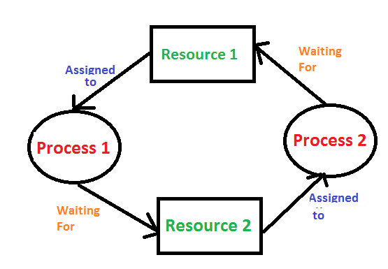
This is a classical example of deadlock in operating systems.
Using gang-scheduling helps preventing deadlocks, because it enforces a global enqueueing order across multiple FIFO queues, instead of letting each queue handling tasks separately.
The paper also mentions allowing device (e.g. GPUs) to execute tasks concurrently can prevent deadlocks. This is because concurrency eliminates the non-preemption property which is required for deadlocks to happen.
If each devices allows concurrency executions (each device has multiple queues), then the task on one queue can be preemptied to allow the other task start executing, thus no deadlock (this is not strictly the case, the post explains an interesting scenario in NCCL where deadlocks can still happen if there are too many communications).